Being an ecologist is all about the trade-off between effort, and time and money. Given infinite amounts of both, we would undoubtedly sample the heck out of nature. But it would be an exercise in diminishing returns: after a certain amount of sampling, we would fail to unturn any stone that has not already been unturned. Thus, ecology is a balancing act of effort: too little, and we have no real insight. Too much, and we’ve wasted a lot of time and money.

I’m always looking for ways to improve my balance, which is why I was interested to see a new paper in Ecology Letters called “Measures of precision for dissimilarity-based multivariate analysis of ecological communities” by Marti Anderson and Julia Santana-Garcon.

In a nutshell, the paper introduces a method for, “assessing sample-size adequacy in studies of ecological communities.” Put in a slightly different way, the authors have devised a technique for determining when additional sampling does not really improve one’s ability to describe whole communities — both the number of species, and their relative abundances. Perfect for evaluating when enough is enough, and adjusting the output of time and money!

In this post, I dig into this technique, show its applications using an example, and introduce a new R function to assess multivariate precision quickly and easily.

Most ecological surveys are concerned with not just one species or the total number of individuals (although some are!). Instead, there is a larger focus on the entire community, and how individuals are distributed among each species within that community. This kind of sampling can be challenging and it’s difficult to tell beforehand exactly how many samples ought to be taken. A pilot study can give you some qualitative insight, but there are rarely hard and fast numbers. Consequently, we err on the side of oversampling.

That’s where the technique by Anderson & Santana-Garcon — called multSE — comes in. It solves the common problem of, as they state:

“How many replicates are needed to sufficiently characterize the community being sampled with reasonable precision for subsequent dissimilarity-based multivariate analysis?”

In other words, if you’re interested in conducting, say, an NMDS, how many samples will need to be taken before you’ve essentially captured the community structure? After what points do more samples become redundant?

Calculating MultSE

The multSE actually based on the age-old idea of sums-of-squares (SS). Unlike an ANOVA, where SS are calculated as the summed squared difference between each point and the overall mean, the multSE is concerned with the summed squared distance between each point in multivariate community space and the centroid (essentially the mean of multivariate space).

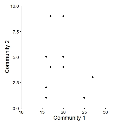
Consider two communities, each of which have 8 species (the same species appear in both communities). We can plot these communities in two-dimensional space, with the axes defined by the communities and the species plotted based on their abundances within each:

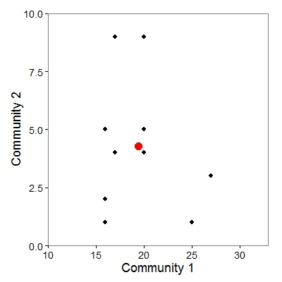
For this cloud of points representing the 8 species in each community, we can calculate a centroid (red point), whose position is defined the average abundance across all species in a given community:

Now connect each species (black points) to the centroid (red point) with a line:

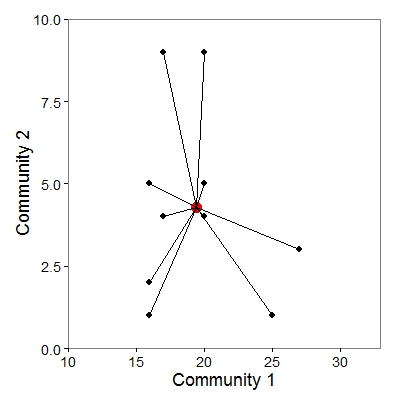
The lines represent the distances. To get the SS of squares, simply add up the squared distances represented by the endpoints of the lines, divided by the total number of points:

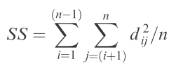
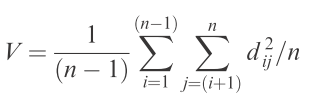
Ta-da! You’ve just calculated the SS used in the calculation of multSE. To derive the estimate of (pseudo-) variance in multivariate space, simply divide by (n – 1):

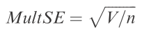
And finally, to get standard error, divide this pseudo-variance by n and take the square-root:

Actually fairly straightforward, and not any more complicated than doing a simple ANOVA. The hardest part, of course, is getting the multivariate distance, which can be obtained from a dissimilarity matrix — for instance, based on Bray-Curtis distances.

So how does this tell us about precision? Well, as more samples are added, they presumably add some degree of similar information about the community. Thus, as the number of samples increases, there exist more and more points closer to that centroid (which will also shift depending on the configuration of points in multivariate space). In terms of the equation above, then, we find with increased sampling the average distance between each point and the centroid gets smaller and smaller. Eventually, new samples will not change the position of the majority of points in that space, or the centroid. After that point, there is no further minimization in multivariate error. In other words, we have discovered the number of samples after which continued sampling will fail to yield any significant improvement in precision.

To derive errors for estimates of multSE — so we can actually test for significant changes in precision as a function of sample size — we can use what Anderson & Santara-Garcon call a ‘double resampling method.’ Without going into too much detail, this involves permutations over some number of iterations — say 10,000 — to arrive at a mean for each sample size, and bootstrapping to derive 95% confidence intervals around these means. This allows us to test whether precision significantly changes from one sample size to another by determining whether the confidence intervals overlap.

I should note that it was brought to my attention in the comments that the use of sums-of-squares to investigate community variances is not a novel idea, and was presented nearly twenty years ago in the literature by Pillar and Orlóci (see references below). In fact, Anderson herself proposed that it can be used to approximate multivariate dispersion some 10 years ago, and thus can be used to test homogeneity of variance among groups in multivariate space (see here, and the betadisper function in the vegan package). That minimizing sums-of-squared distances had endured beyond simple ANOVA well into the 21st century and the wide adoption of multivariate techniques to address complex community structures is a testament to its utility and interpretability.

An Illustrated Example

So, how does one interpret the output from these equations?

To begin, let’s use an example. I’ll draw on some fish survey data from Poor Knight’s Island and included as a supplement to the article above. Briefly, the data were collected using visual census along a 25 x 5 m transect at a depth of 8-20 m. Three time periods were sampled: September 1998 (n = 15), March 1999 (n = 21), and September 1999 (n = 20).

Naturally, we’ll be using an R function to perform the calculations. I actually re-wrote the function included with the supplements (MSEgroup.d) to make it more efficient. The new function is called multSE and allows the analysis to be parsed by multiple groups — in this case, sampling periods, but it could just as easily be different sites, treatments, etc. The latest versions of these functions can be found at my GitHub repository: https://github.com/jslefche/multSE.

First, we need to load the function from Github:

# Load multSE function
library(devtools)
multSE = source_url("https://raw.githubusercontent.com/jslefche/multSE/master/R/multSE.R")[[1]]

Next, we need to import the data:

# Poor Knights fish survey data, from supplementary material
tf = tempfile()
download.file("https://raw.githubusercontent.com/jslefche/multSE/master/data/PoorKnights.csv", tf)
pk = read.csv(tf)

The first column represents the sample number, the second the sampling period, followed by abundance data for 47 species observed on the surveys.

Now, we need to create a species-by-community distance matrix. Here, Anderson and Santana-Garcon use a Bray-Curtis distance. Note the data have been log(x + 1) transformed:

# Load vegan library
library(vegan)
# Create species-by-site distance matrix
D = vegdist(pk[,3:49] + 1)

Finally, supply the distance matrix D to the multSE function, and define the groups (sampling periods):

# Run multSE function
(output = multSE(D, group = factor(pk$Time)))

The output gives the group (sampling period), the number of bootstrapped samples (1, 2, …, n) and the mean pseudo-variance. These are followed by columns for the lower and upper 95% confidence intervals based on 10,000 bootstrapped / permuted values (the default).

A more intuitive way to explore these results is by graphing them:

# Plot output
library(ggplot2)
 
ggplot(output, aes(x = n.samp, y = means, group = group)) +
  geom_errorbar(aes(ymax = upper.ci, ymin = lower.ci), width = 0.2)+
  geom_point(aes(shape = group, fill = group), size = 4) + 
  scale_shape_manual(values = c(21, 24:25), name = "")+
  scale_fill_manual(values = c("black","grey50","white"), name = "")+
  coord_cartesian(ylim = c(0, 0.65)) +
  theme_bw(base_size = 18) +
  labs(x = "Sample size (n)", y = "Multivariate pseudo SE") +
  theme(legend.position = c(0.8, 0.8), 
        panel.grid.major = element_blank(), 
        panel.grid.minor = element_blank())

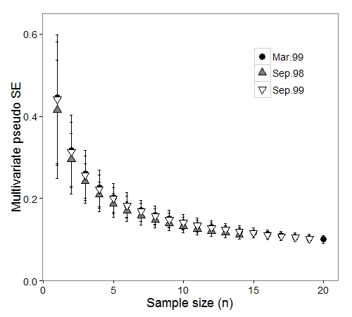
This plot is analogous to Figure 2b in the Anderson & Santana-Garcon paper (although they have removed a few points along the beginning of the x-axis).

As expected, mean error decreases (and precision increases) as more samples are taken. The errors around those means also decrease with more samples. But the multivariate standard error starts to level out around n = 10 samples.

If we consider the sampling period with the most samples — March 1999 — we can place a horizontal line at the multivariate SE for the largest sample size (n = 21). By tracing it backwards, we can pinpoint the exact number of samples where the confidence intervals last overlap this line:

It is immediately clear that one can take only n = 14 samples and not see a significant decline in precision: This is a one-third reduction in effort! That means less SCUBA, less boat time, fewer personnel. Significant savings!

Anderson & Santana-Garcon go on to show how complex designs can be summarized into a single measure of multivariate precision by extracting the residuals from a PERMANOVA. I won’t go into the math but you can access this output by switching the argument permanova = T in the multSE function, which produces the following output:

(output2 = multSE(D, nresamp = 10000, group = factor(pk$Time), permanova = T))
 
ggplot(output2, aes(x = n.samp, y = means)) +
  geom_errorbar(aes(ymax = upper.ci, ymin = lower.ci), width = 0.2)+
  geom_point(size = 4) + 
  # coord_cartesian(ylim = c(0, 0.65)) +
  theme_bw(base_size = 18) +
  labs(x = "Sample size (n)", y = "MultSE based on residual mean square") +
  theme(legend.position = c(0.8, 0.8), 
        panel.grid.major = element_blank(), 
        panel.grid.minor = element_blank())

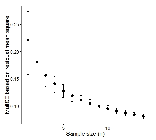
Which is analogous to Figure 3 in the Anderson and Santana-Garcon paper. In this case, we can estimate the change in precision with an increasing number of samples across all sampling periods, and come to much the same conclusion: there is no significant gain in precision after n = 14 samples.

(I should note that the functions included in the supplements of the Anderson & Santana-Garcon paper — multSE.group.d or multSE.d — should generate very similar outputs, but are considerably slower for large numbers of iterations than multSE. See here for examples.)

When is multSE useful?

As pointed out in the paper, this is useful in designing studies to optimize sampling effort. This can be done by running a pilot survey, sorting a bunch of samples, and calculating multSE, then going back and collecting only enough samples to satisfying the minimum level of precision identified during the pilot. Of course, the danger here is that the community does not change between when the pilot was conducted, and when the actual surveying occurs.

Anderson and Santana-Garcon also point out that there is no universal threshold for multSE — it depends only on the communities studied during the time and area at which the samples were taken. So it isn’t useful to extrapolate inferences from one survey at one time and place to another survey at another time and place.

I actually came at this from a slightly different perspective. I’ve been working up some long-term survey data, and earlier sampling dates had fewer surveys. I wanted to understand if this might be a problem — if those communities could have been undersampled relative to the later sampling dates in terms of defining community structure.

Either way, this stands to be a powerful tool for understanding how to allocate sampling effort in ecological surveys.

References

Anderson, MJ and J Santanta-Garcon. 2015. “Measures of precision for dissimilarity-based multivariate analysis of ecological communities.” Ecology Letters 18(1): 66-73.

Orlóci, L. & Pillar, V.D. 1989. “On sample size optimality in ecosystem survey.” Biometrie Praximetrie 29: 173-184.

Pillar, V.D. & Orlóci, L. 1996. “On randomization testing in vegetation science: multifactor comparisons of relevé groups.” Journal of Vegetation Science 7: 585-592.