
Recently, I was exploring techniques to interpolate some missing environmental data, and stumbled across something called ‘random forest’ analysis. Random what now? I did a little digging and came across the massive and insanely complicated field of machine learning. I couldn’t find a concise guide to machine learning techniques, or when I might want to use one or the other, so I thought I would cobble together a brief guide on my own. Below is a rough stab at explaining and exploring different machine learning techniques, from CARTs to GBMs, using R.
Before I get started, I should add the disclaimer that I’m not a statistician and have no formal training in any of these techniques, so what follows is my attempt to synthesize across book chapters, papers, web pages, blog posts, questions on Stackexchange, and YouTube videos (there are a surprising number of YouTube videos of supremely esoteric statistical lectures). My goal was to create a brief, comprehensible, and most of all practical introduction to regression trees and machine learning — the questions I felt I wanted answered when I first started exploring, but couldn’t find in a single spot. That said, if anyone finds any mistakes (of which there are sure to be many!), please let me know and I’ll integrate into the following.
What is machine learning?
Learning is, in its most basic form, the appropriation of knowledge, which can then be used to contextualize existing knowledge and to modify behavior. (Hey, you just learned something!)
Machine learning is the idea that machines can use new data (knowledge) to change its structure or program and increase its performance. In the case of ecology, we are often interested in prediction: it’s why nearly every paper these days reports on a linear model (or structural equation model!). Thus, the point of machine learning is to use new data to improve predictive ability.
There are three implications in the above statement. First, that there is some base level of performance, and thus there is already some knowledge available with which to generate an initial set of predictions (known as deductive learning). Second, that performance can be evaluated, and therefore improvement can be identified. Think of this like rejiggering your model to raise the goodness-of-fit. Finally, that the process is iterative: the model must be continually challenged with new knowledge in order to improve.
Machine learning is often supervised: in other words, you have some input and output in mind, and you want to constrain the model to fit the variables you measured and think are important. This is in contrast to unsupervised learning, in which the model aggregates the data based on patterns in the data itself (think: cluster analysis).
Why machine learning?
Supervised machine learning techniques are most analogous to traditional linear modeling used in ecology, but with several important differences:
- They can handle responses of any type (continuous, categorical)
- They do not require normality. In other words, they make no assumptions about the underlying distribution of some theoretical population
- They do not impose linearity. Thus, they are ideal for predicting relationships that are highly non-linear
- They are insensitive to differences in units, transformations, outliers, and correlations among variables
- Interactions among predictors are automatically modeled
- They seldom choose irrelevant predictors
- Some techniques can accommodate missing data, both in the response and in the predictors
They do, however, have some drawbacks:
- They are prone to overfitting (particularly if care is not taken)
- They do not return an effect size, so there is no single summary metric that can be reported and compared
Let’s begin by exploring the root (pun intended) of machine learning, the Classification and Regression Tree.
Putting the CART before the lm: Classification and Regression Trees
Classification and regression trees (CARTs), sometimes called decision trees, work by repeatedly splitting the response data into two groups that are as homogeneous as possible. The split is determined by the single predictor that best discriminates among the data. The binary splits continue to partition the data into smaller and smaller groups, or nodes, until the groups are no longer homogeneous. This effort produces a single tree where the binary splits form the branches and the final groups compose the terminal nodes, or leaves. The tree is a referred to as a classification tree if the leaves are levels of a categorical variable, or a regression tree if the leaves represent values of a continuous variable.
The model decides which variable to split on based on impurity, or how similar points are within a group. If all points are identical, then impurity is zero, and increases as points become more dissimilar. Thus, maximizing homogeneity is a matter of minimizing impurity. Impurity is calculated differently for different kinds of trees. For classification trees, impurity is most often measured by the Gini index, which reflects the proportion of responses in each level of a categorical variable. The Gini index is small when many observations fall into a single category, so the split is made at the single variable which minimizes the Gini index. For regression trees, impurity is most commonly measured by the sum of squares around the groups means. Thus, as in a least squares linear model, the split is made at the variable that minimizes the root-mean-squared error.
So how does the model decide when to stop? Presumably you could continue to build out the tree until every leaf is a single observation. Another way to phrase this question is: how do you prevent the model from overfitting the data? The answer is: pruning. Pruning is the act of overgrowing the tree and then cutting it back. Ultimately pruning should yield a tree that optimizes the trade-off between complexity and predictive ability.
Pruning begins by creating a nested series of trees of increasing number of leaves, from 0 (no splits) to however many can be reasonably obtained from the data. For each number of leaves, an optimal tree can be recovered, i.e., one that minimizes the overall misclassification rate or the total residual sum-of-squares for a given leaf size (the mean squared error, MSE). To choose among these nested trees–to select the tree of optimal size–we conduct a cross-validation procedure. For a given tree size, cross-validation divides the data into equal portions, removes one portion from the data, builds a tree using the remaining portion, and then calculates the error between the observed data and the predictions. This procedure is repeated for each of the remaining portions and then the overall error is summed across all subsets of the data. This is done for each of the nested trees. The tree of optimal size is then determined based on the smallest tree that is with in 1 standard error of the minimum error observed across all trees.
Let’s see how this works by building a simple classification tree. We’ll use the iris dataset that is ubiquitous in statistical programs. iris measures four morphological characters–sepal length and width, and petal length and width–for each of 50 observations of three species of irises: Iris setosa, I. versicolor, and I. virginica. It is included in the base package of R. Here’s a quick look at the data:
Now let’s build a classification tree to see how the morphological characters relating to sepals and petals predict the species of iris. There are a few packages in R that perform CART analysis. Let’s use the most straightforward one, rpart. Once we load the package the function we are interested in the rpart function, which is constructed identically to most other basic modeling functions in R, with a model statement (y ~ x) followed by the data:
The output from the function reports the tree in text format:
n= 150

node), split, n, loss, yval, (yprob)
      * denotes terminal node

1) root 150 100 setosa (0.33333333 0.33333333 0.33333333)
  2) Petal.Length< 2.45 50   0 setosa (1.00000000 0.00000000 0.00000000) *
  3) Petal.Length>=2.45 100  50 versicolor (0.00000000 0.50000000 0.50000000)
    6) Petal.Width< 1.75 54   5 versicolor (0.00000000 0.90740741 0.09259259) *
    7) Petal.Width>=1.75 46   1 virginica (0.00000000 0.02173913 0.97826087) *
We can see that the first split is on Petal.Length, with all 50 observations of I. setosa having a Petal.Length less than 2.45 cm. further splits are on Petal.Width, where almost all I. versicolor having a Petal.Width < 1.75 cm. and almost all I. virginica having a Petal.Width >= 1.75 cm. Of course this would be easier to show graphically, which we can do quite easily:

We can go back and investigate how these splits were made by exploring the raw data. Plotting the first splitting variable, Petal.Length, we can easily see how I. setosa cleanly separates from the other two species:

And then within the second node (upper part of the panel above containing I. versicolor and I. virginica), we see again a very clean split on Petal.Width ,with only a few miscategorizations:

Note how the unimportant variables, Sepal.Width and Sepal.Length, are no where to be found in this tree. Again, machine learning is very good at identifying and ignoring unimportant variables. Also note that the tree has self-pruned, in this case based on the cost-complexity parameter (the default is 0.1. You can change this to be more or less stringent depending on your needs).
You can call up information on the pruning procedure, as well as overall model fit, by using the function printcp:
> printcp(tree.model)

Classification tree:
rpart(formula = Species ~ Sepal.Length + Sepal.Width + Petal.Length +
    Petal.Width, data = iris)

Variables actually used in tree construction:
[1] Petal.Length Petal.Width

Root node error: 100/150 = 0.66667

n= 150

    CP nsplit rel error xerror     xstd
1 0.50      0      1.00   1.14 0.052307
2 0.44      1      0.50   0.69 0.061041
3 0.01      2      0.06   0.08 0.027520
The most important column here is xerror, which is the cross-validation error. It really only makes sense when we grow the tree a bit more:
> tree.model.updated = update(tree.model, control = rpart.control(minsplit = 2))
> printcp(tree.model.updated)

Classification tree:
rpart(formula = Species ~ Sepal.Length + Sepal.Width + Petal.Length +
    Petal.Width, data = iris, control = rpart.control(minsplit = 2))

Variables actually used in tree construction:
[1] Petal.Length Petal.Width

Root node error: 100/150 = 0.66667

n= 150

    CP nsplit rel error xerror     xstd
1 0.50      0      1.00   1.19 0.049592
2 0.44      1      0.50   0.79 0.061150
3 0.02      2      0.06   0.08 0.027520
4 0.01      3      0.04   0.09 0.029086
We’ve grown out the tree by setting the minimum number of observations at each split to be 2 (in other words, there need to be only 2 observations in a group for a split to be attempted). We can see from the table that there is no improvement in the cross-validation error when moving from 2 to 3 splits (in fact, the model gets slightly worse). Hence why the original function returned only 2 splits (first on Petal.Length, then on Petal.Width).
You may come across another package in R that does CART, party. Instead of pruning based on some index of impurity, they actually perform a conditional test of independence at each split. In other words, they ask if the response (iris species) is independent of the covariates (petal and sepal length and width) at each split by conducting permutation tests: randomly shuffling observations around for each variable and asking if the observed data better predict the response than the permuted data, based on a comparison of P-values. If not, they continue splitting. If so, they stop growing the tree.
The function to conduct this kind of CART analysis is ctree, and has the same formulation as rpart:

You can see that this function produces a slightly more complex tree, as well as a slightly prettier plot. The first split is again on Petal.Length and then Petal.Width but there is a final split again on Petal.Length, all of which are highly significant. There are also histograms under each leaf showing the proportion of observations that fall into each of the three species ta the terminal nodes.
So the question is, which to use: rpart or ctree? rpart tends to be biased towards variables with many possible splits or many possible values, whereas ctree is not. ctree also is based on statistical stopping rules (e.g., P < 0.05) whereas rpart is based on an somewhat meaningless threshold of impurity.
Power in numbers: Ensembles and Bagging
Even with pruning, a single CART is likely to overfit the data, particularly when there are many potential splits and/or many predictors, and thus is not very good for prediction. One way to get around this is to build a bunch of trees on only subsets of the data, and generalize across them. Because any given tree is constructed with only a portion of the data, the likelihood of overfitting is drastically reduced. Moreover, averaging across many trees is likely to wash out any spurious signals from a single tree. This is the idea of ensemble learning, or combining many ‘weak learners’ (individual trees) to produce one ‘strong learner’ (the ensemble).
The idea of taking a portion of the data and using it to build many trees is called bagging. Its a fairly straightforward process for a categorical variable:
- Take a sample of size N from the data with replacement (a bootstrapped sample)
- Build a tree but do not prune
- Store the tree and assign a class to each ‘observation’ based on the leaf in which it falls
- Repeat 1-3 K times (say, 500)
- For each observation, count the number of times it is assigned to a given class and divide by the total number of trees
- Final assignment to a class is by majority vote across all trees (e.g., if an observation is assigned to Class 1 more than 50% of the time, it’s called a “1”)
A continuous variable is even more straightforward:
- Take a sample of size N from the data with replacement (a bootstrapped sample)
- Build a tree but do not prune
- Store the tree and assign each observation the mean of the leaf in which it falls
- Average the assigned means across all trees in which the observation appears
Bagging helps reduce the so-called ‘bias-variance tradeoff.’ Suppose there is some universal true value that we are trying to predict using our model; bias is the degree to which our predictions differ from this true value. Variance is the degree to which those predictions differ from each other. This idea is often illustrated with a bulls-eye (and in unmixed company, with urinals):
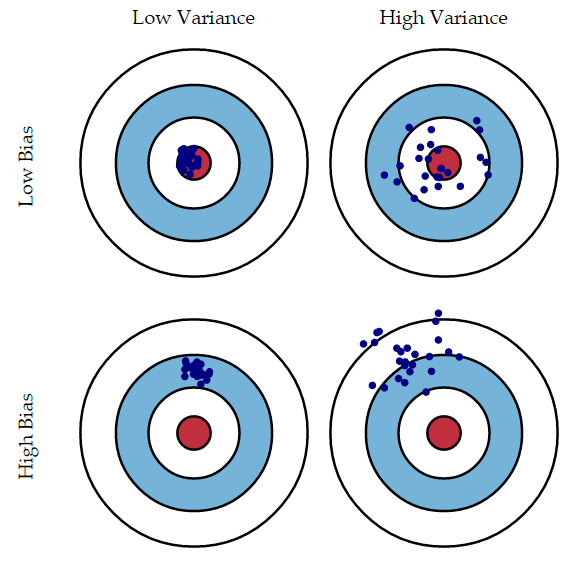
We have no idea what the bias of our trees are because we don’t know what the truth is (in most cases). But by generating and averaging across many trees, we can reduce the variance, particularly as we add more and more trees (see a simple statistical explanation of this phenomenon here).
Another benefit of using only a (bootstrapped) portion of the data is that the remaining data, called the out-of-bag (‘OOB’) sample, can be used to provide an independent (‘honest’) estimate of how well the model performs. This is done by challenging each tree with the OOB sample and either tallying the number of misclassifications, or, for continuous variables, calculating the mean square error (MSE). The overall OOB error for the ensemble is the mean of the proportion of misclassifications, or the MSE. If these values are high, then the models do poorly when faced with ‘new’ data and thus are probably not good for prediction.
The major problem with bagging is that the same predictors are used for all trees, so the improvement from tree-to-tree can only vary so much. In other words the trees are correlated, which can increase the variance of the averaged predictions. This led to the development of a slightly altered technique, the random forest analysis.
Seeing the forest from the trees: Random Forests
Random forests (RFs) are, as the name implies, an ensemble of trees that are built using a special variant of bagging. Like bagging, RFs use a bootstrapped sample of the data to construct the model. But they also use only a proportion of the predictors (typically the square root of the total number of predictors.) In doing so, the trees are truly independent from one another (decorrelated), reducing the bias-variance tradeoff and making RFs a much more accurate alternative to bagging. Another interesting feature is that by subsampling both the data and the predictors, RFs can be fit to more predictors than there are observations, which seems counterintuitive at first but may be of real interest for ecological experiments, which typically suffer from low replication.
Let’s apply the random forest approach to the iris dataset. We call on the package randomForest and the function (surprise) randomForest:
> library(randomForest)
> (RF.model = randomForest(Species ~ Sepal.Length + Sepal.Width + Petal.Length + Petal.Width, data = iris))

Call:
 randomForest(formula = Species ~ Sepal.Length + Sepal.Width +      Petal.Length + Petal.Width, data = iris)
               Type of random forest: classification
                     Number of trees: 500
No. of variables tried at each split: 2

        OOB estimate of  error rate: 4%
Confusion matrix:
           setosa versicolor virginica class.error
setosa         50          0         0        0.00
versicolor      0         47         3        0.06
virginica       0          3        47        0.06
We see first the type of random forest: classification, which makes sense because our response is categorical (species). The output also reports the number of trees in the forest (500) and the number of predictors sampled at each split (2). Next is the OOB error rate, which is only 4% (quite low!). Finally, the confusion matrix, which shows the number of misclassifications (none for I. setosa and 3 each for I. versicolor and I. virginica).
Unlike a single CART, random forests do not produce a single visual, since of course the predictions are averaged across many hundreds or thousands of trees. So calling the plot function does not return a tree as above, but instead this:

This plot shows how the OOB error rate (proportion of misclassifications) for each of the three species changes with the size of the forest (the number of trees). Obviously with few trees the error rate is high, but as more trees are added you can see the error rate decrease and eventually flatten out.
When building random forests, there are three tuning parameters of interest: node size, number of trees, and number of predictors sampled at each split. Careful tuning of these parameters can prevent extended computations with little gain in error reduction. For example, in the above plot, we could easily reduce the number of trees down to 300 and experience relatively little loss in predictive ability:
update(RF.model, ntree = 300)

Call:
 randomForest(formula = Species ~ Sepal.Length + Sepal.Width +      Petal.Length + Petal.Width, data = iris, ntree = 300)
               Type of random forest: classification
                     Number of trees: 300
No. of variables tried at each split: 2

        OOB estimate of  error rate: 4.67%
Confusion matrix:
           setosa versicolor virginica class.error
setosa         50          0         0        0.00
versicolor      0         47         3        0.06
virginica       0          4        46        0.08
You can see there was only a 0.67% increase in the OOB error rate when going from 500 to 300 trees. For such a small dataset the trade-off between computation time (number of trees) and OOB error is so minimal that you could run the RF with 10,000 trees in the blink of an eye and really be confident in your predictions, but for larger datasets it may be worth building the forest up slowly and checking the above plot to see when the error begins to flatten out.
One parameter worth additional tuning is the number of predictors tried at each split . I have found the train function in the caret package to be extremely useful in exploring optimal values for this parameter, and others. train tries a number of different parameters, compares the error rates among the forests, and suggests the smallest parameter that generates an appreciable decrease in error rate.
> library(caret)
> train(Species ~ Sepal.Length + Sepal.Width + Petal.Length + Petal.Width, data = iris, method = "rf")
Random Forest

150 samples
  4 predictor
  3 classes: 'setosa', 'versicolor', 'virginica'

No pre-processing
Resampling: Bootstrapped (25 reps)

Summary of sample sizes: 150, 150, 150, 150, 150, 150, ...

Resampling results across tuning parameters:

  mtry  Accuracy   Kappa      Accuracy SD  Kappa SD
  2     0.9428538  0.9132775  0.03565227   0.05397453
  3     0.9435548  0.9143132  0.03386990   0.05130329
  4     0.9421559  0.9121565  0.03554293   0.05404513

Accuracy was used to select the optimal model using  the largest value.
The final value used for the model was mtry = 3.
This function will take a while as the forest needs to be built again and again for multiple levels of mtry (the parameter in randomForest corresponding to the number of variables tried at each split). Eventually, though, it reveals mtry = 3 to be yield the greatest accuracy, so we can re-run our RF using update(RF.model, mtry = 3), but there is no appreciable reduction in error so we can leave it be for now. This may not always be the case, though, so it’s worth exploring. For the record, the default number of splits at each node is the square-root of the total number of predictors for classification trees, and the number of predictors divided by 3 for regression trees.
Despite not yielding a single visualizable tree, one of the major advantages of random forests is that they can provide a measure of relative importance. By ranking predictors based on how much they influence the response, RFs may be a useful tool for whittling down predictors before trying another framework, such as CART of linear models. Importance can be obtained using the importance function, and plotted using the varImpPlot function:
> importance(RF.model)
             MeanDecreaseGini
Sepal.Length         8.849666
Sepal.Width          1.979043
Petal.Length        45.694857
Petal.Width         42.683772
> varImpPlot(RF.model)

The table reports the mean decrease in the Gini Index, which if you recall, is a measure of impurity for categorical data. For each tree, each predictor in the OOB sample is randomly permuted (aka, shuffled around) and passed to the tree to obtain the error rate (again, Gini index for categorical data, MSE for continuous). The error rate from the unpermuted OOB is then subtracted from the error rate on the permuted OOB data, and averaged across all trees. When this value is large, it implies that a variable had a strong relationship with the response (aka, the model got much worse at predicting the data when that variable was permuted). The plot communicates the same data as in the table, with points farther along the x-axis deemed more important. As we already knew, Petal.Length and Petal.Width are the two most important variables. (For continuous variables, the function will return a second column, the total increase in node impurities, but you should really focus on the mean decrease in the Gini index or % increase in MSE. See a comparison of the two importance statistics here.)
One other useful aspect of random forests is getting a sense of the partial effect of each predictor given the other predictors in the model. (This has analogues to partial correlation plots in linear models.) This is done by holding each value of the predictor of interest constant (while allowing all other predictors to vary at their original values), passing it through the RF, and predicting the responses. The average of the predicted responses are plotted against each value of the predictor of interest (the ones that were held constant) to see how the effect of that predictor changes based on its value. This exercise can be repeated for all other predictors to gain a sense of their partial effects.
The function to calculate partial effects is partialPlot. Let’s look at the effect of Petal.Length:
partialPlot(RF.model, iris, "Petal.Length")

The y-axis is a bit tricky to interpret. Since we are dealing with classification trees, its on the logit scale, so its the probability of success. In this case, the partial plot has defaulted to the first class, which represents I. setosa. This plot says that there is a high chance of successfully predicting this species from Petal.Length when Petal.Length is less than around 2.5 cm, after which point the chance of successful prediction drops off precipitously. This is actually quite reassuring as this is the first split identified way back in the very first CART (where the split was < 2.45 cm).
When responses are continuous it is tempting to interpret the y-axis literally: i.e., the effect of X and a given level of X. However, because of averaging, this is not quite true. Thus partial dependency plots are best interpreted with language such as: “The effect of X becomes more negative as X becomes large,” without referring to specific magnitudes. It is also useful for making qualitative comparisons among predictors: “The effect of X becomes more negative as X becomes large for class A than for class B.” In other words, the y-axis is a relative scale, and should not be reported literally.
Its worth noting that the default behavior of randomForest is to refuse to fit trees with missing predictors. You can, however, specify a few alternative arguments: the first is na.action = na.omit, which removes the ros with missing values outright. Another option is to use na.action = na.roughfix, which replaces missing values with the median (for continuous variables) or the most frequent level (for categorical variables). Missing responses are harder: you can either remove that row, or use the function rfImpute to impute values. The imputed values are the average of the non-missing observations, weighted by their proximity to non-missing observations (based on how often they fall in terminal nodes with those observations). rfImpute tends to give optimistic estimates of the OOB error.
Learn from your mistakes
Random forests are one of the best classifiers, perhaps the best, but there is one other variant that is gaining considerable attention: boosting. It is also an ensemble learning technique, relying on many weak learners to average out to be a strong learner. But unlike bagging and RFs, boosting focuses on poor or hard to predict responses.
Like random forests, boosted models grow the forest tree by tree. But instead of randomly sampling the data, boosted models use all of the data to compute the first tree. The second tree then attempts to predict the residuals (or misclassifications) of the first tree (here’s where focusing on the errors comes into play!). The third tree predicts the error of the second tree, and so on sequentially for some number of trees, averaging across all predictions at the end.
Now where does the ‘gradient’ part of the name come into play? The answer has to do with which tree is added next to the ensemble, and is a bit tricky. For each tree, we can set up a linear equation to adjust our predicted values to minimize the overall error of the ensemble, otherwise referred to as the ‘loss function.’ The parameters of the loss function are identified using a procedure called ‘gradient descent,’ which iteratively searches parameter space for values that minimize error. Each iteration brings the values closer to this minima, hence the descent (moving towards the minima) and gradient (each iteration). A simple explanation of this phenomenon can be found here. The next tree added is the one which minimizes the loss function. Given that I am not a mathematician I find this part of GBMs most troublesome, so I point readers to this YouTube video for a better (and likely more accurate) explanation of this procedure.
The benefit of boosting is that it produces more accurate results, even better than random forests. The bad part of this approach is that it is seriously prone to overfitting, drilling down to explain every last bit of residual error. So what to do? Well, we can actually introduce a term that limits the amount that each subsequent tree can vary from the previous trees, called shrinkage. Shrinkage cripples the learning rate, preventing the model from explaining too much too quickly. It also prevents a single extreme prediction from monopolizing the direction of the ensemble.
The gbm function in the gbm package is constructed identically to randomForest:
> library(gbm)
> (GBM.model = gbm(Species ~ Sepal.Length + Sepal.Width + Petal.Length + Petal.Width, data = iris))

Distribution not specified, assuming multinomial ...

gbm(formula = Species ~ Sepal.Length + Sepal.Width + Petal.Length +
    Petal.Width, data = iris)
A gradient boosted model with multinomial loss function.
100 iterations were performed.
There were 4 predictors of which 3 had non-zero influence.
As with RFs, however, the output is largely uninteresting, summarizing only aspects of the procedure.
The caret package is once again useful here, as it will tune not only shrinkage but also the number of trees and another parameter, known as tree complexity. This is the number of interactions considered at each split: a complexity of 1 would indicate an additive model, 2 would include all two-way interactions, and so on. We can run train our GBM to evaluate the optimal set of parameters:
>train(Species ~ Sepal.Length + Sepal.Width + Petal.Length + Petal.Width, data = iris, method = "gbm", verbose = F)

Stochastic Gradient Boosting

150 samples
  4 predictor
  3 classes: 'setosa', 'versicolor', 'virginica'

No pre-processing
Resampling: Bootstrapped (25 reps)

Summary of sample sizes: 150, 150, 150, 150, 150, 150, ...

Resampling results across tuning parameters:

  interaction.depth  n.trees  Accuracy   Kappa      Accuracy SD  Kappa SD
  1                   50      0.9465926  0.9190737  0.02748061   0.04181538
  1                  100      0.9429930  0.9136046  0.02511809   0.03824108
  1                  150      0.9416093  0.9115102  0.02621297   0.03986666
  2                   50      0.9436937  0.9147320  0.02832516   0.04292142
  2                  100      0.9414723  0.9113837  0.03092802   0.04679108
  2                  150      0.9408710  0.9104459  0.02573531   0.03901087
  3                   50      0.9443783  0.9156623  0.02557269   0.03898993
  3                  100      0.9373647  0.9051849  0.03256986   0.04934706
  3                  150      0.9359724  0.9030440  0.02974680   0.04514420

Tuning parameter 'shrinkage' was held constant at a value of 0.1
Accuracy was used to select the optimal model using  the largest value.
The final values used for the model were n.trees = 50, interaction.depth = 1 and shrinkage = 0.1.
It appears that we gain no improvement in accuracy by building larger ensembles (N = 150 trees), or including two- or three-way interactions. Note, however, that train fixes shrinkage at 0.1. We may wish to consider even more values of shrinkage, but there is a tradeoff: as shrinkage declines, the less improvement there can be from tree to tree, and the longer it will take to build out the ensemble. Let’s try again but this time force train to evaluate a few different levels of shrinkage (this will take some time!):
> train(Species ~ Sepal.Length + Sepal.Width + Petal.Length + Petal.Width, data = iris, method = "gbm", verbose = F,
+ tuneGrid = expand.grid(n.trees = c(50, 100, 150), interaction.depth = c(1:3), shrinkage = c(0.001,0.01,0.1)))

Stochastic Gradient Boosting

150 samples
  4 predictor
  3 classes: 'setosa', 'versicolor', 'virginica'

No pre-processing
Resampling: Bootstrapped (25 reps)

Summary of sample sizes: 150, 150, 150, 150, 150, 150, ...

Resampling results across tuning parameters:

  shrinkage  interaction.depth  n.trees  Accuracy   Kappa      Accuracy SD  Kappa SD
  0.001      1                   50      0.9505802  0.9251849  0.02926160   0.04419113
  0.001      1                  100      0.9541243  0.9305533  0.02766876   0.04171652
  0.001      1                  150      0.9533970  0.9294674  0.02602863   0.03925257
  0.001      2                   50      0.9512369  0.9262396  0.02744372   0.04135652
  0.001      2                  100      0.9499567  0.9242752  0.02317560   0.03492588
  0.001      2                  150      0.9490595  0.9229470  0.02657233   0.04005263
  0.001      3                   50      0.9535015  0.9296373  0.02868207   0.04322973
  0.001      3                  100      0.9526661  0.9283826  0.02581713   0.03891843
  0.001      3                  150      0.9512392  0.9262340  0.02729566   0.04114082
  0.010      1                   50      0.9527567  0.9285264  0.02469789   0.03721730
  0.010      1                  100      0.9562467  0.9337958  0.02488327   0.03752349
  0.010      1                  150      0.9554720  0.9325758  0.02523049   0.03808975
  0.010      2                   50      0.9528695  0.9286925  0.02457375   0.03702163
  0.010      2                  100      0.9549469  0.9317775  0.02332391   0.03526206
  0.010      2                  150      0.9556467  0.9328117  0.02330619   0.03528697
  0.010      3                   50      0.9529340  0.9287460  0.02427634   0.03663929
  0.010      3                  100      0.9534353  0.9294664  0.02288978   0.03460840
  0.010      3                  150      0.9556221  0.9327479  0.02218689   0.03358392
  0.100      1                   50      0.9519167  0.9271580  0.02413783   0.03637932
  0.100      1                  100      0.9505814  0.9251653  0.02259921   0.03407646
  0.100      1                  150      0.9477770  0.9209154  0.02349076   0.03547047
  0.100      2                   50      0.9527017  0.9283512  0.02568497   0.03880646
  0.100      2                  100      0.9521672  0.9275389  0.02713360   0.04101317
  0.100      2                  150      0.9506557  0.9252175  0.02604625   0.03937270
  0.100      3                   50      0.9527081  0.9282722  0.02286232   0.03471801
  0.100      3                  100      0.9498015  0.9239354  0.02195031   0.03321223
  0.100      3                  150      0.9492606  0.9231135  0.02389194   0.03612641

Accuracy was used to select the optimal model using  the largest value.
The final values used for the model were n.trees = 100, interaction.depth = 1 and shrinkage = 0.01.
As before, the most accurate GBM had 100 trees and an interaction depth of 1, but in this case the slightly lower value of shrinkage (0.01 vs 0.1) gave a slightly more accurate result.
As with randomForest, we can easily get an estimate of variable importance:

Here, the relative influence refers to the contribution of each variable in minimizing the loss function. It is calculated by averaging the number of times a variable is selected for splitting weighted by the squared improvement to the model as the result of each split. It is then scaled so the values sum to 100. Here we again see Petal.Length and Petal.Width as having the most explanatory power, as with the RF analysis.
We can also derive partial dependency plots, as before:
plot(GBM.model, "Petal.Length")
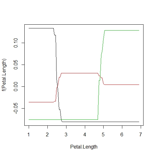
Again we see that the probability of successfully predicting species based on Petal.Length is very high for I. setosa for Petal.Length < 2.45 cm but, interestly, it is equally high for predicting I. virginica when Petal.Length > 5.05 cm.
A drawback of GBMs is that they must be fit sequentially, because they depend on the results of the previous tree. Random forests, on the other hand, can be fit in parallel (say, by sending some chunk of trees to a multicore computer). Thus, the forest can, in theory, be grown much more quickly for RFs than for GBMs, depending on the number of trees, size of the dataset, and the speed of the computer.
Unlike random forests, GBMs handle missing values in the predictors by default. They actually produce a hidden, or surrogate, split at every node to bin missing values. Then if the tree is challenged with data that are missing a variable, the split is decided based on the surrogate variable (typically one that has a high correlation with non-missing observations).
Now what?
So when should you use these techniques? It depends on the goals of your analysis, and the size and complexity of your dataset. Here’s a quick table to help you decide:
| Type | Data Size | Data Complexity | Visuali-zation | Accuracy | Variable Importance |
Computation Time |
| CART | Small (best) | Low (best) |
Yes | Low | No | Very low |
| Random forests | Any | Any | No | High | Yes | Low (if parallelized) |
| Gradient boosted models | Any | Any | No | Highest | Yes | High |
For most ecological datasets, which are generally small (hundreds to tens of thousands of observations), things like computation time may not be an issue. Ultimately, I recommend gradient boosted models (GBMs). To me, they make intuitive sense. If you were taking a test and the question had two parts, why throw out your answers for the first part before you go on to the second? But its vitally important to explore and tune GBMs, since overfitting is such an issue.
I didn’t hit many topics, including stochastic gradient models (which combine the random subsampling procedure of random forests with gradient boosting), Adaboost (the precursor to gradient boosting), and other complex topics. If there is something you would like to see explained, or something I got wrong above, let me know in the comments and I’ll work on it. Happy analyzing!
Further Reading
De’ath, G., and Fabricius, K. E.. (2000). Classification and regression trees: A powerful yet simple technique for ecological data analysis. Ecology 81:3178–3192.
Cutler, D. Richard, et al. (2007). Random forests for classification in ecology. Ecology 88(11): 2783-2792.
Elith, J., Leathwick, J. R. and Hastie, T. (2008). A working guide to boosted regression trees. Journal of Animal Ecology 77: 802–813.
Model Training and Tuning (caret)

Thanks for this Jon. I am actually interested in several of these techniques for some of my current projects.
Great introduction to machine learning in ecology, thanks!
I recently found your blog and I love it. I am a microbiologist, working on soil bacterial communities and have struggled with the ecology and statical backgrounds (since I’m NOT trained in any of this). I find you post super useful, and although I am not an R professional, I manage running the scripts with your annotations (thank A LOT for this).
I was working on RF models – not classification but regression trees (since I am using bacterial abundances) and it works nicely and the results are great. However, one quick question (since I am not a statistician): You’ve been commenting on the y-axis in partial dependency plots, being the probability of success (of prediction) for classification trees. Now my question is how to interpret this axis for regression trees – i guess its still a probability of success – but I get an axis raging e.g. from 0.18 – 0.28. So can I actually say the probability of success is a certain value (based on my y-axis)?
I hope this is not to much of a dumb question.
Thanks again Jon 🙂
Hi Krissey, thanks for checking out my post. For regression trees, the partial plots are (as far as I understand it) the change in the effect (what I interpret as the linear coefficient) with a corresponding change in the predictor. So I would interpret as the effect gets more positive, less positive, etc as the predictor increases. Hope this helps! Cheers, Jon
The best explanation of machine learning jargons for an experimental biologist. Thanks for putting this together.
Thanks Jon, this is really useful as an intro to machine learning tools in R.
Thanks Jon! I was also in the phase of meeting with machine learning through the random forest!! But instead of searching and synthesizing I came across your post!!!
Many thanks!!!
You are a life safer! I literally was struggling for 2 days now, to understand the precision of RF method until i found this posting. Thank you so much!
Thank you much for your help..A very clear and comprehensive explanation with the application of R. i really appreciate that. One remaining question: How do you see classical statistical techniques and machine learning techniques being used together to complement each other for analysis of ecological data?
Good question…I definitely see machine learning as a variable selection tool to identify the important predictors, which you can then carry through into more classic predictive techniques. Cheers, Jon
“The binary splits continue to partition the data into smaller and smaller groups, or nodes, until the groups are no longer homogeneous” This is not exactly true. Actually, the more you split, the more the groups are homogeneous. The stopping criterion is more that the new groups do not bring “important” new information, in other words, the new group are not “a lot” more homogeneous than the old one.
Hope this helps,
Cheere
Hi,
I am trying to do NMDS plot for microbial amplicon data.I used below code to generate NMDS plot, but I used here raw OTU count as input. but normalized data is preferred for NMDS as input, could you please suggest how I can normalize like rank threshold transformation or any other method.
prev.ordNMDS_data1 <- ordinate(data1, "NMDS", "bray") plot_ordination(data1, ordination = prev.ordNMDS_data1, color="Region") + theme_minimal() + geom_point(size=5)
Thanks
Yogesh
Very clear and extremely useful for ecologists interested in machine learning, thanks a lot !
Short question: Are there any updated references (since you wrote the post in 2015) that you would recommand ?
Nope, none that I have seen!