The other day, I posted an introductory demo to mapping in R using some of the built-in maps. But of course there are only a few regions represented in the “maps” package: the US states, the US as a whole, Italy, France, and the world. Even then, there are some limitations to these: for instance, the USSR is still alive and kicking in the world of “maps.” If you are living in the 21st century–or working somewhere other than these locations–you may want to supply your own, more updated maps. The most popular filetype is, of course, the GIS shapefile. But to access, visualize, manipulate, and plot on shapefiles, it was formerly necessary to use ArcGIS, which is proprietary and thus costly. I’ll show you how to do it all in R!
In the next installment of this series, I’ve shown how to import, manipulate, and visualize GIS shapefiles in R using the same LTER data using the world shapefile publicly available at: http://aprsworld.net/gisdata/world/. Its necessary to download and extract the directory containing the GIS files, and set the working directory to point R to those files on your computer. The goal of this exercise is similar to the first part: plot the global LTER sites on the world map and shade the countries in which they occur.
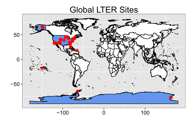
library(ggplot2) #Calls: fortify, ggplot
library(rgdal) #Calls: readOGR
library(sp) #Calls: spTransform

# First, download and extract the "world" shapefile from:
# http://aprsworld.net/gisdata/world/

# Read in the shapefile using the function `readOGR`
world=readOGR(".",layer="world")
# The first argument is the location, the second is the name of the shapefile

# The world of course is not a plane, but an ellipse
# Additionally, the earth's surface is not perfectly smooth
# Consequently, lat/long coordinates need to be "projected" onto an
# irregular ellipse
# This information is stored in the proj4string, which in this case is provided with
# the shapefile
print(proj4string(world))
# +proj is the type of project, +ellips is the ellipse that is used, and
# +datum is the irregularity of the earth's surface
# One can switch between ellipses and datums using the function `spTransform`
world2=spTransform(world,CRS("+proj=latlong +ellips=GRS80"))
# Where CRS defines the target projection
# The type of projection depends on the geographical location and the size of
# the study area

# Now read in the coordinates of global LTER sites from:
# http://www.lternet.edu/sites/coordinates
sites=read.delim(textConnection(" 	0 	0
  Andrews Forest LTER (AND) 	44.21 	-122.26
  Arctic LTER (ARC) 	66.63 	-149.60
  Baltimore Ecosystem Study (BES) 	39.10 	-76.30
  Bonanza Creek LTER (BNZ) 	64.86 	-147.85
  California Current Ecosystem LTER (CCE) 	32.87 	-120.28
  Cedar Creek LTER (CDR) 	45.40 	-93.20
  Central Arizona - Phoenix LTER (CAP) 	33.43 	-111.93
  Coweeta LTER (CWT) 	35.00 	-83.50
  Florida Coastal Everglades LTER (FCE) 	25.47 	-80.85
  Georgia Coastal Ecosystems LTER (GCE) 	31.43 	-81.37
  Harvard Forest LTER (HFR) 	42.53 	-72.19
  Hubbard Brook LTER (HBR) 	43.94 	-71.75
  Jornada Basin LTER (JRN) 	32.62 	-106.74
  Kellogg Biological Station LTER (KBS) 	42.40 	-85.40
  Konza Prairie LTER (KNZ) 	39.09 	-96.58
  LTER Network Office (LNO) 	35.08 	-106.62
  Luquillo LTER (LUQ) 	18.30 	-65.80
  McMurdo Dry Valleys LTER (MCM) 	-77.00 	162.52
  Moorea Coral Reef LTER (MCR) 	-17.49 	-149.83
  Niwot Ridge LTER (NWT) 	39.99 	-105.38
  North Temperate Lakes LTER (NTL) 	46.01 	-89.67
  Palmer Antarctica LTER (PAL) 	-64.77 	-64.05
  Plum Island Ecosystems LTER (PIE) 	42.76 	-70.89
  Santa Barbara Coastal LTER (SBC) 	34.41 	-119.84
  Sevilleta LTER (SEV) 	34.35 	-106.88
  Shortgrass Steppe (SGS) 	40.83 	-104.72
  Virginia Coast Reserve LTER (VCR) 	37.28 	-75.91 "),header=F,strip.white=T)
sites=droplevels(sites[-1,]); names(sites)=c("sites","lat","long")

# Convert sites to SpatialPoints object with same projection as world map
sites_sp=SpatialPoints(sites[,c(3,2)],proj4string=CRS(proj4string(world)))
# Use function `over` to obtain a list of SpatialPolygons that contain the sites
index=over(sites_sp,world)
# Note that some entries are NAs because they fall outside of the polygons
# defined by the map
# Return the region names of the SpatialPolygons containing each site
region_names=rownames(world@data[world@data$NAME %in% index$NAME,])

# Create a dataframe for plotting from the shapefile
world.fort=fortify(world) #This may take some time
# And add a column "fill" denoting whether the site is present in the region
world.fort$fill=ifelse(world.fort$id %in% region_names,"true","false")

# Use ggplot to plot the dataframe as a polygon
ggplot()+
  # Fill the region polygons where fill=="true" and set country borders to "black"
  geom_polygon(data=world.fort,aes(x=long,y=lat,group=group,fill=fill),col="black")+
  # Set the fill colors
  scale_fill_manual(values=c("white","cornflowerblue"))+
  # Plot the individual sites as red dots
  geom_point(data=sites,aes(x=long,y=lat),col="red",size=4,alpha=0.9)+
  # Set labels
  labs(x="",y="",title="Global LTER Sites")+
  # Set base theme and remove legend, and fill grid with grey background
  theme_bw(base_size=18)+theme(legend.position="none",
  panel.background=element_rect(fill="grey90"))

# Note that Antarctica is not shaded. This is because the lat/long coordinates fall
# offshore of the continent
# We can jimmy one of the points (Palmer LTER) to actually put it on the continent
sites[22,2]=sites[22,2]+0.04

# And repeat:
# Convert sites to SpatialPoints object with same projection as world map
sites_sp=SpatialPoints(sites[,c(3,2)],proj4string=CRS(print(proj4string(world))))
# Use function `over` to obtain a list of SpatialPolygons that contain the sites
index=over(sites_sp,world)
# Return the region names of the SpatialPolygons containing each site
region_names=rownames(world@data[world@data$NAME %in% index$NAME,])

# And add a column "fill" denoting whether the site is present in the region
world.fort$fill=ifelse(world.fort$id %in% region_names,"true","false")

# Use ggplot to plot the dataframe as a polygon
ggplot()+
  # Fill the region polygons where fill=="true" and set country borders to "black"
  geom_polygon(data=world.fort,aes(x=long,y=lat,group=group,fill=fill),col="black")+
  # Set the fill colors
  scale_fill_manual(values=c("white","cornflowerblue"))+
  # Plot the individual sites as red dots
  geom_point(data=sites,aes(x=long,y=lat),col="red",size=4,alpha=0.9)+
  # Set labels
  labs(x="",y="",title="Global LTER Sites")+
  # Set base theme and remove legend, and fill grid with grey background
  theme_bw(base_size=18)+theme(legend.position="none",
  panel.background=element_rect(fill="grey90"))
