For decades, biologists and ecologists have largely characterized biological diversity using metrics based on entropy, a concept rooted in information theory that suggests one can quantify the degree of uncertainty associated with predicting bits and pieces of information. In ecology, this has boiled down to determining whether species drawn from a community are the same or different. The metrics will sound familiar to anyone who has taken an introductory ecology class–the Shannon index, Simpson diversity–but Lou Jost, Anne Chao, and others have highlighted the fact that the non-linearity of these indices may lead researchers to grossly misinterpret the underlying diversity of the community in question.
Consequently, Lou Jost proposed in 2006 that diversity values be converted into equivalent or effective numbers of species (also known as Hill numbers), which is the number of equally abundant species necessary to produce the observed value of diversity (an analogue the concept of effective population size in genetics). Converting the entropic indices into effective numbers yield values of diversity that are intuitive and behave as we would expect–for instance, effective numbers obey the doubling property, which states that if two communities with X equally abundant but totally distinct species are combined, then the diversity of the combined community should be twice that of the original communities, or 2X. Moreover, they are in units of “number of species” and thus values of diversity are comparable across different metrics.
Below is some R code from a recent lecture I gave on quantifying biological diversity. In it, I demonstrate the utility of the two most common metrics of diversity, Shannon and Simpson diversity, the utility of converting them into effective numbers, and show how to derive them from a more general equation for entropy (as well as using the same equation to generate so-called “diversity profiles”). The code uses simulated data so its entirely self contained (no downloads required!).
________________________
First, consider the simplest case: a community with S species, all with equal abundances A. For community 1, S = 500 species, and A = 1 individual of each species. For community 2, S = first 250 species from community 1, and A = 1 individuals of each species.
community1=data.frame(t(rep(1,500))); colnames(community1)=paste("sp",1:500)
community2=data.frame(t(c(rep(1,250)))); colnames(community2)=paste("sp",1:250)
First, let’s calculate the species richness of each community using the `specnumber` function in the `vegan` package, and compare the richness of the two communities
As we know (since we created the communities), the richness of community 2 is half that of community 1.
Now let’s incorporate information on species abundances into our diversity index. We’ll begin with the commonly used Shannon index, which quantifies the uncertainty that any two species drawn from the community are different. Shannon diversity ranges from 0 (total certainty) to log(S) (total uncertainty).
Let’s use function `diversity`, also in the `vegan` package, to calculate Shannon diversity for both communities
H1=diversity(community1,index="shannon"); H1
H2=diversity(community2,index="shannon"); H2
And now let’s ensure that community 1 has the maximum value of Shannon diversity, since it has the maximum number of species with equal numbers of individuals for each species.
H1==log(S1)
And now let’s test the same logical argument as before, asking whether Shannon diversity of community 2 is half that of community 1.
H2==0.5*H1
Uh, ok. So that isn’t true. What the heck is going on here? Let’s do a little exploring.
Let’s calculate Shannon diversity for all levels of species richness from S = 1 to 1000 (this will take a bit), and then plot the results.
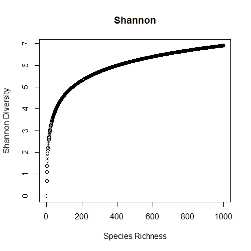
Ah-ha! Here is our answer. The relationship between species richness and Shannon diversity is non-linear: at higher levels of species richness, communities will appear more similar (in terms of the magnitude of the index) that at lower levels of species richness. This is exactly how the index is supposed to behave, but ecologists are used to thinking about species richness, which behaves differently. Thus, Jost points out in a 2010 paper that it is so very tempting to misinterpret these indices, especially at high levels of richness. So what’ s the solution? Convert to effective numbers!
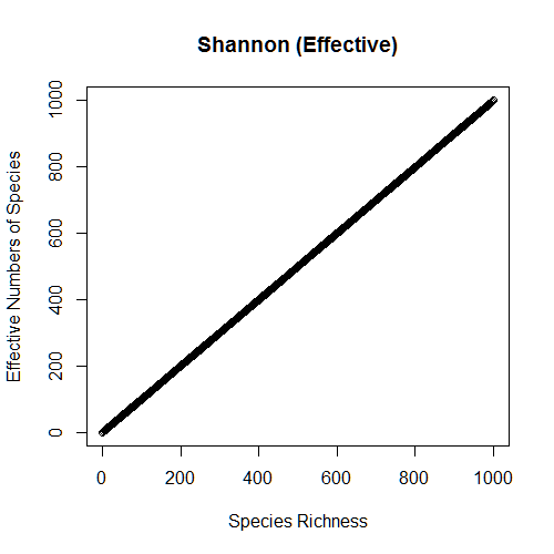
HE1=exp(diversity(community1,index="shannon")); HE1
HE2=exp(diversity(community2,index="shannon")); HE2
as.character(HE2)==as.character(0.5*HE1)

from 1:1000
shannon_effective=matrix(ncol=2,nrow=1000)
for(i in 1:1000) {
  community=data.frame(t(rep(1,i))); colnames(community)=paste("sp",1:i)
  shannon_effective[i,1]=i
  shannon_effective[i,2]=exp(diversity(community,index="shannon")) }
plot(shannon_effective[,1],shannon_effective[,2],xlab="Species Richness",
ylab="Effective Numbers of Species",main="Shannon (Effective)")
And now we arrive at values of Shannon diversity that behave like species richness: effective Shannon diversity of community 2 is now half that of community 1. This is because the index has been linearized!
Let’s repeat this exercise with another popular index, Simpson diversity (or Gini-Simpson diversity).
D1=diversity(community1,index="simpson"); D1
D2=diversity(community2,index="simpson"); D2

simpson=matrix(ncol=2,nrow=1000)
for(i in 1:1000) {
  community=data.frame(t(rep(100,i))); colnames(community)=paste("sp",1:i)
  simpson[i,1]=i
  simpson[i,2]=diversity(community,index="simpson") }
plot(simpson[,1],simpson[,2],xlab="Species Richness",ylab="Simpson Diversity",
main="Simpson")

DE1=1/(1-D1); DE1
DE2=1/(1-D2); DE2
DE2==0.5*DE1

simpson_effective=matrix(ncol=2,nrow=1000)
for(i in 1:1000) {
  community=data.frame(t(rep(100,i))); colnames(community)=paste("sp",1:i)
  simpson_effective[i,1]=i
  simpson_effective[i,2]=1/(1-diversity(community,index="simpson")) }
plot(simpson_effective[,1],simpson_effective[,2],xlab="Species Richness",
ylab="Effective Numbers of Species",main="Simpson (Effective")
The output from the above code shows that Simpson diversity saturates at much lower levels of richness than Shannon diversity, which exacerbates the issue of misinterpretation.
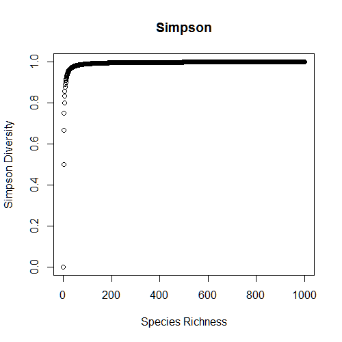
But once again, effective numbers transformation linearizes this index.

Both Shannon and Simpson diversity are special cases entropy, which is the measure of disorder in a system (more disorder = more diversity). There is a general equation for entropy from which Shannon and Simpson diversity are derived.
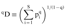 This equation has a parameter q that defines its sensitivity to rare species: low values of q favor rare species, high values of q favor abundant species. For example, Shannon diversity is of order q = 1, and for Simpson diversity q = 2. When q = 0, diversity = S (richness), because rare species are treated the same as abundant ones.
One cool thing that can be done with this equation is that one can calculate diversity along a continuum of values of q to create what is called a ‘diversity profile’. A diversity profile allows you to judge the contributions of rare vs abundant species in a community.
# The following function `divprof` calculates the diversity from this equation along
# a continuum of q values
divprof=function(community) {
  cbind(
    seq(0,5,by=0.11),
    unlist(lapply(seq(0,5,by=0.11),function(q) sum(apply(community,1,function(x)
       (x/sum(x))^q))^(1/(1-q))))) }

community1.divprof=divprof(community1)
plot(community1.divprof[,1],community1.divprof[,2],ylim=c(0,500),pch=16,cex=2,
xlab="q value",ylab="Diversity")
A diversity profile is not really informative when all species are equally abundant:
So let’s create a third community with 500 species whose abundances are randomly sampled from 1 to 1,000.
set.seed(9)
community3=data.frame(t(sample(1:1000,500))); colnames(community3)=paste("sp",1:500)
# Apply function `divprof` to this community
community3.divprof=divprof(community3)
plot(community3.divprof[,1],community3.divprof[,2],pch=16,cex=2,xlab="q value",
ylab="Diversity")
# Where q=0, diversity is species richness
text(0.6,501,labels=c("Richness"))
points(community3.divprof[1,1],community3.divprof[1,2],col="red",pch=16,cex=2)
# Where q=1, diversity is Shannon diversity
exp(diversity(community3,index="shannon"))
text(2,exp(diversity(community3,index="shannon"))+5,labels=c("Shannon Diversity"))
points(community3.divprof[10,1],community3.divprof[10,2],col="red",pch=16,cex=2)
# Where q=2, diversity is Simpson diversity
1/(1-diversity(community3,index="simpson"))
text(3.9,1/(1-diversity(community3,index="simpson"))-12,
labels=c("Simpson Diversity"))
points(community3.divprof[28,1],community3.divprof[28,2],col="red",pch=16,cex=2)
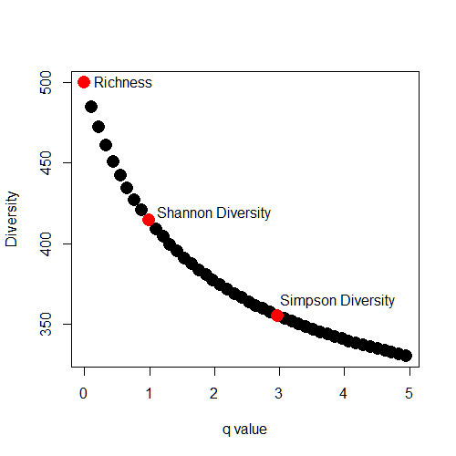
The diversity profile for this community shows the values of richness, Shannon diversity, and Simpson diversity, and tells us what we already knew: there is strong dominance in this community.
The full code (annotated, with another example) is available below.
References:
Jost, L. 2006. Entropy and diversity. Oikos 113(2): 363-375.
Leinster, T. and C.A. Cobbold. 2012. Measuring diversity: the importance of species similarity. Ecology 93(3): 477-489.
________________________
FULL CODE:
# First, consider the simplest case: a community with S species, all with equal abundances A
# For community 1, S = 500 species, and A = 1 individual of each species
# For community 2, S = first 250 species from community 1, and A = 1 individuals of each species
community1=data.frame(t(rep(1,500))); colnames(community1)=paste("sp",1:500)
community2=data.frame(t(c(rep(1,250)))); colnames(community2)=paste("sp",1:250)

# Load vegan package, which contains many useful functions for calculating diversity
# install.packages("vegan")
library(vegan)

# First, let's calculate the species richness of each community using the `specnumber` function
S1=specnumber(community1); S1
S2=specnumber(community2); S2
# We know this is true because we created these two communities to have 500 and 250 species each
# Furthermore, we know that the diversity in community 2 is half that of community 1
S2==0.5*S1

# Now let's incorporate information on species abundances
# We'll begin with the commonly used Shannon index, which quantifies the uncertainty that any two species
# drawn from the community are different
# Shannon diversity ranges from 0 (total certainty) to log(S) (total uncertainty)

# Let's use function `diversity` to calculate Shannon diversity for both communities
H1=diversity(community1,index="shannon"); H1
H2=diversity(community2,index="shannon"); H2
# Community 1 has equal representation of all 500 species, so H1 should be equal to log(S)
H1==log(S1)
# Community 2 has equal represention of only 250 species, so we might expect H2 to equal half of H1
H2==0.5*H1
# Hmm...let's investigate this further

# Let's calculate Shannon diversity for all levels of species richness from S = 1 to 1000 (this will take a bit)
shannon=matrix(ncol=2,nrow=1000)
for(i in 1:1000) {
  community=data.frame(t(rep(1,i))); colnames(community)=paste("sp",1:i)
  shannon[i,1]=i
  shannon[i,2]=diversity(community,index="shannon") }
# And plot the results
plot(shannon[,1],shannon[,2],xlab="Species Richness",ylab="Shannon Diversity",main="Shannon")
# The relationship between richness and Shannon diversity is non-linear! Hence why H2 is not half of H1

# The concept of 'effective numbers' solves this issue by imposing a linear transformation on Shannon diversity
# Effective numbers are the number of equally abundant species necessary to produce the observed
# value of diversity
# Effective numbers range from 1 to S, where a value of S would indicate all species are present and
# in equal abundances

# The conversion of Shannon diversity to effective numbers is exp(H)
HE1=exp(diversity(community1,index="shannon")); HE1 # This is what we expect given what we know about Community 1
HE2=exp(diversity(community2,index="shannon")); HE2 # And this is also what we expect
# And now diversity of community 2 is exactly half of the diversity of community 1!
as.character(HE2)==as.character(0.5*HE1)
# This outcome of effective numbers is known as the 'doubling property'

# Calculate effective numbers of species (from Shannon diversity) for all levels of species richness from 1:1000
shannon_effective=matrix(ncol=2,nrow=1000)
for(i in 1:1000) {
  community=data.frame(t(rep(1,i))); colnames(community)=paste("sp",1:i)
  shannon_effective[i,1]=i
  shannon_effective[i,2]=exp(diversity(community,index="shannon")) }
plot(shannon_effective[,1],shannon_effective[,2],xlab="Species Richness",ylab="Effective Numbers of Species",main="Shannon (Effective)")
# This relationship is now linear!

# Let's use another common diversity index: Simpson diversity
# Simpson diversity is 1-probability that any two species drawn from the community are the same
# Simpson diversity ranges between 0 (100% probable) and 1 (0% probable)
# We will again use the `diversity` function from the vegan package
D1=diversity(community1,index="simpson"); D1
D2=diversity(community2,index="simpson"); D2
# YIKES! These values are nearly identical, yet we know community 2 is half as diverse as community 1!

# Again, let's calculate Simpson diversity for all levels of species richness from 1 to 1000
simpson=matrix(ncol=2,nrow=1000)
for(i in 1:1000) {
  community=data.frame(t(rep(100,i))); colnames(community)=paste("sp",1:i)
  simpson[i,1]=i
  simpson[i,2]=diversity(community,index="simpson") }
plot(simpson[,1],simpson[,2],xlab="Species Richness",ylab="Simpson Diversity",main="Simpson")
# Non-linear relationships saturates at very low levels of richness, leading to the misleading
# values from our two communities

# Once again, effective numbers to the resuce!
# The conversion of Simpson diversity to effective numbers is 1/1-D
DE1=1/(1-D1); DE1
DE2=1/(1-D2); DE2
# The metric produces the same values of diversity as Shannon diversity: this is because abundances are equal
DE2==0.5*DE1 # And, as we expected, diversity in community 2 is half of that in community 1

# Calculate effective numbers of species (from Simpson diversity) for all levels of species richness from 1:1000
simpson_effective=matrix(ncol=2,nrow=1000)
for(i in 1:1000) {
  community=data.frame(t(rep(100,i))); colnames(community)=paste("sp",1:i)
  simpson_effective[i,1]=i
  simpson_effective[i,2]=1/(1-diversity(community,index="simpson")) }
plot(simpson_effective[,1],simpson_effective[,2],xlab="Species Richness",ylab="Effective Numbers of Species",main="Simpson (Effective")
# Like the conversion of Shannon diversity, effective numbers from Simpson diversity yields a linear relationship
# with species richness

# Both Shannon and Simpson diversity are special cases entropy = the measure of disorder in a system
# (more disorder = more diversity)
# There is a general equation for entropy from which Shannon and Simpson diversity are derived
# This equation has a parameter `q` that defines its sensitivity to rare species
# Low values of q favor rare species, high values of q favor abundant species
# When q = 0, diversity = S (richness), because rare species are treated the same as abundant ones

# The following function `divprof` calculates the diversity from this equation along a continuum of q values,
# creating what is called a 'diversity profile'
# Diversity profiles allow you to gauge the relative contribution of rare species to diversity your system
divprof=function(community) {
  cbind(
    seq(0,5,by=0.11),
    unlist(lapply(seq(0,5,by=0.11),function(q) sum(apply(community,1,function(x) (x/sum(x))^q))^(1/(1-q))))) }

# Let's apply function `divprof` to our community of species with equal abundances
community1.divprof=divprof(community1)
plot(community1.divprof[,1],community1.divprof[,2],ylim=c(0,500),pch=16,cex=2,xlab="q value",ylab="Diversity")
# Not very interesting, since there are neither rare nor abundant species--every species is present in equal numbers,
# and therefore diversity is the same at all levels of q

# Let's create a new community of where abundances of S = 500 species are randomly sampled between 1 - 1000
set.seed(9)
community3=data.frame(t(sample(1:1000,500))); colnames(community3)=paste("sp",1:500)
# Apply function `divprof` to this community
community3.divprof=divprof(community3)
plot(community3.divprof[,1],community3.divprof[,2],pch=16,cex=2,xlab="q value",ylab="Diversity")
# Where q=0, diversity is species richness
text(0.6,501,labels=c("Richness"))
points(community3.divprof[1,1],community3.divprof[1,2],col="red",pch=16,cex=2)
# Where q=1, diversity is Shannon diversity
exp(diversity(community3,index="shannon"))
text(2,exp(diversity(community3,index="shannon"))+5,labels=c("Shannon Diversity"))
points(community3.divprof[10,1],community3.divprof[10,2],col="red",pch=16,cex=2)
# Where q=2, diversity is Simpson diversity
1/(1-diversity(community3,index="simpson"))
text(3.9,1/(1-diversity(community3,index="simpson"))-12,labels=c("Simpson Diversity"))
points(community3.divprof[28,1],community3.divprof[28,2],col="red",pch=16,cex=2)
# This plot shows that richness is high, but that as we increasingly favor abundant species (increase q, move to
# the right along the x-axis), diversity drops, indicating that community 3 is composed of some abundant and
# some rare species

# For kicks, let's create a community of 5 very abundant species, and 450 very rare species
set.seed(6)
community4=data.frame(t(c(sample(500:1000,5),sample(1:5,495,replace=T))))
colnames(community4)=paste("sp",1:500)
# Apply function `divprof` to community 4
community4.divprof=divprof(community4)
plot(community4.divprof[,1],community4.divprof[,2],pch=16,cex=2,xlab="q value",ylab="Diversity")
text(0.45,25,labels=c("Richness")) #Where q=0, diversity is species richness
text(2,35+exp(diversity(community4,index="shannon")),labels=c("Shannon Diversity")) #Where q=1, diversity is Shannon diversity
text(3.1,30+1/(1-diversity(community4,index="simpson")),labels=c("Simpson Diversity"))
# Diversity drops off more steeply, since our community is dominated by a few very abundant species!

Thank you! I’ve been lost in the literature about measuring diversity for a week. This provides some much needed clarity.
Good day! I would like to ask if there is a macro or a calculator made specifically for converting Shannon’s index to effective number of species directly? Thank you for your soon reply!
Hi, you can try the script in the post. In lieu, the transformations are quite simple: 1/(1-D) for Simpson, and exp(H) for Shannon. Cheers, Jon
Hi – thank you for your post. Nice and informative. One remark – in the last figure with the diversity profile, you put the simpson index at q=3, but isn´t it usually at q=2 ?
cheers
Whoops, yes, you’re correct!
Thank you for this post! In the example above, it seems that the Hill’s index ends up converting the diversity index to species richness (1:1 relationship). Will this always be the case, and if so, why not just use species richness?
Hi Ryan, this is only true if individuals are equally distributed among species (as in the example). In nature this is rarely so, so the equivalency will not hold in such cases. HTH, Jon