[Updated December 30, 2019: You can read more about the package, new functionality, and other approaches to SEM in my online book (work-in-progress): https://jslefche.github.io/sem_book/]
[Updated October 13, 2015: Active development has moved to Github, so please see the link for the latest versions of all functions: https://github.com/jslefche/piecewiseSEM/]
Nature is complex. This seems like an obvious statement, but too often we reduce it to straightforward models. y ~ x and that sort of thing. Not that there’s anything wrong with that: sometimes y is actually directly a function of x and anything else would be, in the words of Brian McGill, ‘statistical machismo.’
But I would wager that, more often that not, y is not directly a function of x . Rather, y may be affected by a host of direct and indirect factors, which themselves affect one another directly and indirectly. If only there was someway to translate this network of interacting factors into a statistical framework to better and more realistically understand nature. Oh wait, structural equation modeling.
What is structural equation modeling?
Structural equation modeling, or SEM for short, is a statistical framework that, ‘unites two or more structural models to model multivariate relationships,’ in the words of Jim Grace. Here, multivariate relationships refers to the sum of direct and indirect interactions among variables. In practice, it essentially strings together a series of linear relationships.
These relationships can be represented using a path diagram with arrows denoting which variables are influencing (and influenced by) other variables. Take a very simple path diagram:

Which is described by the equation: Y ~ X1 + X2.
Not consider a different arrangement of the same variables:
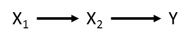
Which is now described by two equations: X2 ~ X1 and Y ~ X2. These two equations make up the SEM.
Assumptions of SEM
There are a few important points to make:
(1) As I pointed out, I’m talking about linear relationships. There are ways to integrate non-linear relationships into SEM (see Cardinale et al. 2009 for an excellent example), but for the most part, we’re dealing with straight lines.
(2) Second, we assume that the relationships above are causal. By causal, I mean that we have structured our models such that we assume X1 directly affects Y , and not the other way around. This is a big leap from more traditional statistics where we the phrase ‘correlation does not imply causation’ is drilled into our brains. The reason we can infer causative relationships has to do with the underlying philosophy of SEM. SEM is designed principally to test competing hypotheses about complex relationships.
In other words, I might hypothesize that Y is directly influenced by both X1 and X2 , as in the first example above. Alternately, I might suspect that X1 indirectly affects Y through X2 . I might have arrived at these hypotheses through prior experimentation or expert knowledge of the system, or I may have derived them from theory (which itself is supported, in most cases, by experimentation and expert knowledge).
Either way, I have mathematically specified a series of causal assumptions in a causal model (e.g., Y ~ X1 + X2 ) which I can then test with data. Path significance, the goodness-of-fit, and the magnitude of the relationships all then have some bearing on which logical statements can be extracted from the test: X1 does not directly affect Y , etc. For more information on the debate over causation in SEMs, see chapters by Judea Pearl and Kenneth Bollen.
(3) Third, in the second example, we have not estimated a direct effect of X1 on Y (i.e., there is no arrow from X1 to Y , as in the first example). We can, however, estimate the indirect effect as the product of the effect of X1 on X2 and the effect of X2 on Y . Thus, by constructing a causal model, we can identify both direct and indirect effects simultaneously, which could be tremendously useful in quantifying cascading effects.
Traditional SEM attempts to reproduce the entire variance-covariance matrix among all variables, given the specified model. The discrepancy between the observed and predicted matrices defines the model’s goodness-of-fit. Parameter estimates are derived that minimize this discrepancy, typically using something like maximum likelihood.
Piecewise SEM
There are, however, a few shortcomings to traditional SEM. First, it assumes that all variables are derived from a normal distribution.
Second, it assumes that all observations are independent. In other words, there is no underlying structure to the data. These assumptions are often violated in ecological research. Count data are derived from a Poisson distribution. We often design experiments that have hierarchical structure (e.g., blocking) or observational studies where certain sets of variables are more related than others (spatially, temporally, etc.)
Finally, traditional SEM requires quite a large sample size: at least (at least!) 5 samples per estimated parameter, but preferably 10 or more. This issue can be particularly problematic if variables are nested, where the sample size is limited to the use of variables at the highest level of the hierarchy. Such an approach drastically reduces the power of any analysis, not to mention the heartbreak of collapsing painstakingly collected data.
These violations are dealt with regularly by, for instance, fitting generalized linear models to a range of different distributions. We account for hierarchy by nesting variables in a mixed model framework, which also alleviates issues of sample size. However, these techniques are not amenable to traditional SEM.
These limitations have led to the development of an alternative kind of SEM called piecewise structural equation modeling. Here, paths are estimated in individual models, and then pieced together to construct the causal model. Piecewise SEM is actually a better gateway into SEM because it essentially is running a series of linear models, and ecologists know linear models.
Evaluating Fit in Piecewise SEM: Tests of d-separation
Piecewise SEM is a more flexible and potentially more powerful technique for the reasons outlined above, but it comes with its own set of restrictions. First, estimating goodness-of-fit and comparing models is not straightforward. In traditional SEM, we can easily derived a chi-squared statistic that describes the degree of agreement among the observed and predicted variance-covariance matrices. We can’t do that here, because we’re estimating a separate variance-covariance matrix for each piecewise model.
Enter Bill Shipley, who derived two criteria of model fit for piecewise SEM. The first is his test of d-separation. In essence, this test asks whether any paths are missing from the model, and whether the model would be improved with the inclusion of the missing path(s). To understand this better, we must first define a few terms.
Shipley’s perspective is based on what are known as directed acyclic graphs (DAG), which are essentially path diagrams, as above. Two variables are considered causally dependent if there is an arrow between them. They are causally independent if there is not an arrow between them. Consider the following example:
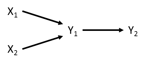
X1 is causally independent of Y2 because no arrow exists between them.
However, X1 indirectly influences Y2 via Y1 . Thus, X1 is causally independent of Y2 conditional on Y1 . This is an important distinction, because it has implications for the way in which we test whether the missing arrow between X1 and Y2 is important.
A test of directional separation (d-sep) asks whether the causally independent paths are significant while statistically controlling for variables on which these paths are conditional. To begin, one must list all the pairs of variables with no arrows between them, then list all the other variables that are direct causes of either variable in the pair. These pairs of independence claims, and their conditional variables, forms the basis set.
For the example above, the basis set is:
X1andX2X1andY2, conditional onY1X2andY2, conditional onY1
The basis set can then be turned into a series of linear models:
X1 ~ X2X1 ~ Y2 + Y1X2 ~ Y2 + Y1
As you can see, we include the conditional variables ( Y1 and Y2 ) as covariates, but we are interested in those missing relationships (e.g., X1 ~ X2). We can run these models, and extract the p-values associated with the missing path, all the while controlling for Y1 and/or Y2. From these p-values, we can calculate a Fisher’s C statistic using the following equation:
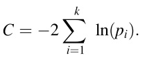
which follows a chi-squared distribution with 2k degrees of freedom (where k = the number of pairs in the basis set). Thus, if a chi-squared tests is run on the C statistic and P < 0.05, then the model is not a good fit. In other words, one or more of the missing paths contains some useful information. Conversely, if P > 0.05, then the model represents the data well, and no paths are missing.
Evaluating Fit in Piecewise SEM: AIC
SEM is often implemented in a model testing framework (as opposed to a more exploratory analysis). In other words, we are taking a priori models of how we think the world works, and testing them against each other: reversing paths, dropping variables or relationships, and so on. A popular way to compare nested models is the use of the Akaike Information Criterion (AIC). Shipley has recently extended d-sep tests to use AIC. It’s actually quite straightforward:
![]()
The formula should look quite familiar if you’ve ever calculated an AIC. In this case, the gobbledy gook in brackets is simply C, above. In this case, however, K is not the number of pairs in the basis set (that’s little k, not big K). Rather, K the number of parameters estimated across all models. The additive term can be modified to provide an estimate of AIC corrected for small sample size (AICc).
An Example from Shipley (2009)
In his 2009 paper, Shipley sets forth an example of tree growth and survival among 20 sites varying in latitude using the following DAG:
![]()
Happily for our purposes, Shipley has provided the raw data as a supplement, so we construct, test, and evaluate this SEM. In fact, I’ve written a function that takes a list of models, performs tests of d-sep, and calculates a chi-squared statistic and an AIC value for the entire model. The function alleviates some of the frustration with having to derive the basis set–an exercise at which I have never reliably performed–and then craft each model individually, which can be cumbersome with many variables and missing paths. You can find the most up to date version of the function on GitHub.
First, we load up the required packages and the data:
Then we load the data and build the model set:
# Load required libraries
library(lmerTest)
library(nlme)

data(shipley2009)

shipley2009.modlist = list(
  lme(DD~lat, random = ~1|site/tree, na.action = na.omit,
    data = Shipley),
  lme(Date~DD, random = ~1|site/tree, na.action = na.omit,
    data = Shipley),
  lme(Growth~Date, random = ~1|site/tree, na.action = na.omit,
    data = Shipley),
  glmer(Live~Growth+(1|site)+(1|tree),
    family=binomial(link = "logit"), data = shipley2009) )
Finally, we can derive the fit statistics:
sem.fit(shipley2009.modlist, shipley2009)
which reveals that C = 11.54 and P = 0.48, implying that this model is a good fit to the data. If we wanted to compare the model, the AIC score is 49.54 and the AICc is 50.08.
*These values differ from those reported in Shipley (2009) as the result of updates to the R packages for mixed models, and the fact that he did not technically correctly model survivorship as a binomial outcome, as that functionality is not implemented in the nlme package. I use the lmerTest package at it returns p-values for merMod objects based on the oft-debated Satterthwaite approximation popular in SAS, but not in R.
Shortcomings of Piecewise SEM
There are a few drawbacks to a piecewise approach. First, the entire issue of whether p-values can be meaningfully calculated for mixed models rears its ugly head once again (see famous post by Doug Bates here). Second, piecewise SEM cannot handle latent variables, which are variables that represent an unmeasured variable that is informed by measured variables (akin to using PCA to collapse environmental data, and using the first axis to represent the ‘environment’). Third, we cannot accurately test for d-separation in models with feedbacks (e.g., A -> B -> C -> A). Finally, I have run into issues where tests of d-separation cannot be run because the model is ‘fully identified,’ aka there are no missing paths. In such a model, all variables are causally dependent. One can, however, calculate an AIC value for these models.
Get to it!
Ultimately, I find SEM to be a uniquely powerful tool for thinking about, testing, and predicting complex natural systems. Piecewise SEM is a gentle introduction since most ecologists are familiar with constructing generalized linear models and basic mixed effects models. Please also let me know if anything I’ve written here is erroneous (including the code on GitHub!). These are complex topics, and I don’t claim to be any kind of expert! I’m afraid I’ve also only scratched the surface. For an excellent introductory resource to SEM, see Jarrett Byrnes’ SEM course website–and take the course if you ever get a chance, its fantastic! I hope I’ve done this topic sufficient justice to get you interested, and to try it out. Check out the references below and get started.
References
Shipley, Bill. “Confirmatory path analysis in a generalized multilevel context.” Ecology 90.2 (2009): 363-368.
Shipley, Bill. “The AIC model selection method applied to path analytic models compared using a d-separation test.” Ecology 94.3 (2013): 560-564.
Shipley, Bill. Cause and correlation in biology: a user’s guide to path analysis, structural equations and causal inference. Cambridge University Press, 2002.

Hello Jon!
Like everyone here, I agree this package is really useful.
I just have one question about the models we can use for semi-continuous zero-inflated data. I was using an approximation with Poisson distribution but a reviewer told me to change for gaussian or gamma (that don’t work because of the zeros). I found that for this kind of data we can use several solutions :
– Tobit regression: assumes that the data come from a single underlying Normal distribution, but that negative values are censored and stacked on zero (e.g. censReg package)
– hurdle or “two-stage” model: use a binomial model to predict whether the values are 0 or >0, then use a linear model (or Gamma, or truncated Normal, or log-Normal) to model the observed non-zero values
– Tweedie distributions: distributions in the exponential family that for a given range of shape parameters (1<p0 (e.g. tweedie, cplm packages)
Does the piecewiseSEM package (version 1.2.1) allow to use one or several of these 3 solutions ?
Thank you for your help!
Best regards,
Isabelle
You should be able to use gamma or negative binomial distributions with `lme4` or `MASS::glmmPQL`. HTH, Jon
Hi Jon — Thanks for your great work. I have been using the current version of the package to fit a model that includes a binomial regression along with normal regressions. Everything works quite well, my only issue is with the calculation of indirect effects. I’ve tried to read all of the responses above, and I know this is an issue that’s been discussed but I don’t see a definitive answer. If I can trouble you again, a cartoon of my model is like this:
A ~ B + C, (binomial)
B ~ E + F, (normal)
C ~ G + H, (normal)
A is a logistic response (it’s presence/absence of insects in patches at a landscape scale, so 0s and 1s, can’t be treated as a proportion). I am interested here in comparing the cascading effects of variables E and G (i.e., which one has a greater indirect effect on A?). So the temptation is multiply the E-to-B coefficient by the B-to-A coefficient, and compare that to G-to-C * C-to-A. Using standardized coefficients, that would be multiplying a coefficient in units of standard deviation with a coefficient on the log odds scale (from the logistic regression).
I wonder if that mixing of units could be acceptable? Even if the units of the product become hard to interpret, it seems to me that I could still answer my question about the relative impact of E and G.
Looking forward to your thoughts!
thanks
Matt
Hey Matt, thanks for reaching out. Comparing the two indirect paths using the product of unstandardized coefficients would be unfair, since the magnitude of the units would affect which is “stronger.” You could definitely compare the unstandardized paths, in which case the standardized coefficient for GLM would follow the equations in Grace et al 2018 Ecosphere. Be sure to take the standard deviation of the link-transformed response AND incorporate the distribution specific variance. HTH, Jon
Dear Jon,
thank you for this great package and the motivating introduction. I want to apply pSEM using mixed models. However I, get the error “Model is recursive. Remove feedback loops!”, although I can’t find any feedback loops in my model:
This is the problematic code piece.
dSep(psem(
lme(oc ~ pla_sp + pla_co + n_till + ph,
random = ~1|vineyard, data = dat.2),
lme(ph ~ oc + pla_co + n_till,
random = ~1|vineyard, data = dat.2),
lme(pla_co ~ n_till,
random = ~1|vineyard, data = dat.2)
))
Do you see the problem in my code. Thanks for help
Regards,
Martin
Hi Martin, Yes it seems you are predicting ph -> oc -> ph (models 1 and 2). Remove that feedback and you should be good to go! HTH, Jon
Hi Jon,
Thanks for your work in this excellent package!
I’m trying to use it to calculate indirect, direct and total effects of several predictor variables which are inter-related (A, B, C, D) on bird counts (which follow a Poisson distribution):
modlist = psem(
lme(T ~ Y + A, random= ~ 1|Site , xy),
lme(S ~ Y + T, random= ~ 1|Site , xy),
glmer(Birds ~ T + A + S + (1|Site), family=”poisson” , xy)
coefs(modlist, xy, standardize = “scale”)
As it has been already discussed here, it seems that is not possible for the current version to calculate standardized coefficients for non-linear responses (besides the new options for binary responses). So this is what I get:
Response Pred Estimate Std.Error DF Crit.Value P.Value Std.Estimate
1 T Y 0.1651 0.0172 69 9.5882 0.0000 0.5796 ***
2 T A -0.0015 0.0003 7 -5.6116 0.0008 -0.6366 ***
3 S Y 1.4978 0.1944 58 7.7058 0.0000 0.6475 ***
4 S T -7.6962 0.6654 58 -11.5654 0.0000 -0.9479 ***
5 Birds T -1.0388 0.2522 80 -4.1180 0.0000 – ***
6 Birds A -0.0022 0.0006 80 -3.5678 0.0004 – ***
7 Birds S 0.0801 0.0347 80 2.3083 0.0210 – *
Since my main interest is to calculate total effects of all variables on bird abundances (which I cannot do like it is because estimates for bird responses are not standardized), I wonder if you think is correct applying the following “manual” calculation considering this formula (from one of your pwpt lessons):
𝛽𝑠𝑡𝑑=𝐵𝑥𝑦∗(𝑠𝑑(𝑥)/𝑠𝑑(𝑦))
In this case, for example, the standardized estimate for the effects of T on Birds would be:
-1.0388 * (sd(xy$T)/sd(xy$Birds) = -1.0388 *(0.3990/2.8568) = -0.1451
A on Birds would be: -0.0022 *(166.6924/2.8568) = -0.1284
And S on Birds would be: 0.0801*(3.2402/2.8568) = 0.0908
If this is correct, I could calculate the indirect effects (for example of Y on Birds) following the normal procedure, that is: (0.5796*-0.1451) + (0.6475*0.0908) + (-0.9479*0.5796*0.0908)= -0.0752
Do you think this approach is valid in the meantime PiecewiseSEM allows to compute the standardized coefficients for Poisson glmer directly? Did I misunderstood the calculation of standardized estimates?
Thanks a lot in advance!
Hi Miguel, Thanks for reaching out. The computation of sd(Birds) is a bit more complicated, since you must take it on the link-transformed data (in this case, you use a log-link) and also incorporate the distribution-specific error for the Poisson distribution. See the Grace et al 2018 paper in Ecosphere. If you do this, the standardized coefficient should be valid. HTH, Jon
Hi Jon,
Thank you very much for this fantastic package that I have used a few times. I’m having a very similar problem to MIGUEL, except that in my case all the models on the psem list have a Poisson distribution with log-link. In order to compute the standardized coefficients for the Poisson glmer I’m following what you do here (to some extent):
https://jslefche.github.io/piecewiseSEM/articles/piecewiseSEM.html
Any idea of what would be the distribution-specific error for the Poisson distribution to be incorporated similarly to what you do with for the binomial distribution based on the link function (adding π^2/3 in this case)?
Many many thanks in advance,
Pedro
Hi Pedro, Sorry for the slow reply! This paper has a nice table with the distribution-specific error variances: Nakagawa, Shinichi, Paul CD Johnson, and Holger Schielzeth. “The coefficient of determination R 2 and intra-class correlation coefficient from generalized linear mixed-effects models revisited and expanded.” Journal of the Royal Society Interface 14.134 (2017): 20170213. HTH, Jon
Hi Jon,
Thank you for your work! This website is extremely helpful and the package is very useful.
My question is whether the Std.Estimate coefficients can be larger than 1 or smaller than -1. My model fit data well and it has high % variance explained and significant coefficients (although I have a small sampling size n=18). Using variance inflation factor (VIF) some of the variables were removed from the model, but I still get some Std.Estimates >1 and <-1.
Thank you for any suggestions,
Best regards,
Oksana
Hi Oksana, Standardization is generally implemented by multiplying the coefficient Beta by the ratio of the standard deviation of x over the standard deviation in y. If the units of Beta are > 1 or < -1, and the standard deviations of x and y are roughly equivalent, then the standardized coefficient can indeed exceed those bounds. HTH, Jon
Thanks Jon, This is very helpful.
Best, Oksana
Hi Jon, I apologise if this has already been answered, I did look through but couldnt find it within the 116 responses to your post. I have specified a pSEM and accounted for failures of directed separation (through specifying correlated errors). Unfortunately my model still hasa poor goodness of fit (p=0.036). What are the next options open to me given this issue? I can (somewhat aribtrarily) remove certain predictor variables from the models resulting in a much better goodness of fit, but this seems to be very unscientific tinkering. Is there an accepted way of stepwise reduction, model averaging or similar to come up with a reduced pSEM model with good fit? Can I just remove each of the non-significant coefficients in turn based on their p values (or perhaps standardized estimate?)?
Hi Jon,
thank you very much for your package, it is really useful.
I just have a question about standardized paths coefficients. As well as other paths, I want to explain plant species richness (which is a count) using glmer and Poisson distribution:
> glmer(Num.diagnostic.sp ~ Coeff.utilization + Cattle.sheep.ratio + Calcareous.substrate + (1 | Region) + (1 | Site), family = poisson, data = db)
I have some circularity warning, but the model runs. The doubt is that in the summary there are not the standardized coefficients for this variable and I need them to build the graph and comparing all the paths with the other variables.
How can I obtain them?
Thank you very much
Francesca
Hi Francesca, Sorry for the slow reply. We are currently working on implementing standardized coefficients for GLM(M) but it is slow going. A bigger issue is circularity in your model. If the model is circular, meaning you have a variable whose paths feed back into that variable, then piecewise SEM is not appropriate. Please email if you want to discuss more! HTH, Jon
Hi Jon, thank you for this package, it’s been a life saver! I’m really enjoying using it to analyse my data. I have one very quick question! I want to be able to compare relative effect among exogenous variables and their indirect effects. I know neither of these two things are possible for non-gaussian data. BUT, the normality rule is that the residuals of your model must be normally distributed, not necessarily your data. so the question is: if my data is not normally-distributed, but the residuals of each individual model in the SEM are, are my standardised coefficients meaningful? (I know this is not an option of binomial, thinking about skewed or other messy distributions).
Thanks!
Hi Felipe, alas the standardized coefficients from GLM(M) are not comparable even if the residuals are normal, as the standard deviation (variance) of the response does not include the link-transformation or the distribution specific variance. We are working to implement this and produce meaningful standardized coefficients (and have done so already for logistic regression) but the process is slow going. I hope to have more updates this summer! HTH, Jon
Hello Jon
I’m confused about the nagelkerke Pseudo R^2 for glm given in the summary of psem in the piecewiseSEM package. I’ve managed to realize that they are the pseudo R^2 for each model independently of the psem. However, they’re so very prone to return a rounded value of 1, even using simple models in the keeley dataset (like a gaussian glm(rich~cover), whereas another package like rcompanion give wildly different results. And I am (was) pretty sure those aren’t overfitted so I’m panicking a bit.
The piecewiseSEM:::rsquared.glm function calculate those a bit differently.from the other (rcompanion::nagelkerke):
In the former it uses the null and residual deviances which are calculated by logLikelihood:
model$null= 2(LL(Saturated Model) – LL(Null Model))
and model$dev = 2(LL(Saturated Model) – LL(Proposed Model))
but are not the same as in the latter, where the nagelkerke seems a bit more by the book (calculating the LL of the model and the null model but not the saturated model as seen here https://stats.idre.ucla.edu/other/mult-pkg/faq/general/faq-what-are-pseudo-r-squareds/)
so, what is the difference? I’m stuck.
and also, just how important are those pseudo Rsquared to tell me “I should not be using this model/I’m using too many parameters”?
Sorry if this is not the correct place for this question or the correct etiquette.
Thank you.
Hi Emerson, I found an issue in the code with computed (pseudo)-R2’s for GLM. I have fixed this in the development version: https://github.com/jslefche/piecewiseSEM/tree/devel Please install and let me know if the issue persists. Sorry about that!
Yes! It all checks out perfectly! Excellent!! Thank you! Also I just updated to R 4.0.1 and still works! Awesome!