Linear mixed effects models are a powerful technique for the analysis of ecological data, especially in the presence of nested or hierarchical variables. But unlike their purely fixed-effects cousins, they lack an obvious criterion to assess model fit.
[Updated October 13, 2015: Development of the R function has moved to my piecewiseSEM package, which can be found here under the function sem.model.fits]
In the fixed-effects world, the coefficient of determination, better known as R2, is a useful and intuitive tool for describing the predictive capacity of your model: its simply the total variance in the response explained by all the predictors in your model.
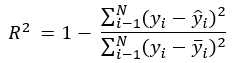
In a least squares regression, R2 is the sum of differences in the observed minus the fitted values, over the sum of the deviation of each observation from the mean of the response, all subtracted from 1:
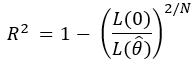
For models estimated using maximum likelihood, this equation was generalized to the ratio of the likelihood of the intercept-only model over the full model, raised to the 2/N, and all subtracted from 1:
Both equations can be interpreted identically.
R2 has a number of useful properties. Its independent of sample size, bound (0,1), and dimensionless, which makes it ideal for comparing fits across different datasets.
I should note, however, that its a poor tool for model selection, since it almost always favors the most complex models. If the goal is to select among the best models, an information criterion approach (such as AIC or BIC) is preferred, since these indicators penalize for the number of predictors.
Unfortunately (and this is a common pitfall), the best model as determined by AIC is not synonymous with a good model. In other words, AIC provides a great test of relative model fit, but not absolute model fit. AIC values are also not comparable across models fit to different datasets. Thus, R2 and AIC both have their place in ecological statistics.
Often, researchers using mixed models report an R2 from a linear mixed model as simply the squared correlation between the fitted and observed values (see here), but this is a pseudo-R2 and is technically incorrect.
Why? Because a mixed effects model yields a variance associated with each random factor and the residual variance, so its not entirely clear which to use when calculating the R2 (the approach above ignores this issue by choosing to calculate R2 relative to only the residual variance, which omits any structure in the data imposed by the random factor).
When hierarchical models with >1 levels are considered, this problem is exacerbated since now we are dealing with variances at multiple levels, plus the residual error. Some people have discussed calculating an R2 value for each level of the random factor, but this can lead to negative R2 values when addition of predictors reduces the residual error while increasing the variance of the random component (or vice versa), even though the sum of the variance components remains unchanged.
So what have we done, historically-speaking? We’ve compared AIC values for the full and null models, or calculated all manner of pseudo-R2s, and quietly (and perhaps for some, ashamedly) went about our business.
Which is why I was so happy to see a paper with the title “A general and simple method for obtaining R2 from generalized linear mixed-effects models” by Shinichi Nakagawa and Holger Schielzeth appear in my newsfeed. Basically, they have derived two easily interpretable values of R2 that address the above issues, specifically that of negative pseudo-R2s with more predictors, while still honoring the random structure of the data.
The first is called the marginal R2 and describes the proportion of variance explained by the fixed factor(s) alone:

The fixed-effects variance is in the numerator. The denominator is the total variance explained by the model, including (in order): the fixed-effects variance, the random variance (partitioned by level l), and the last two terms add up the residual variance and are the additive dispersion component (for non-normal models) and the distribution-specific variance.
The second is the conditional R2, which describes the proportion of variance explained by both the fixed and random factors:

In this case, the numerator contains both the variance of the fixed effects, as well as the sum of random variance components for each level l of the random factor. You’ll note the denominator is identical.
This approach was later modified by Johnson (2014) to include random slope models.
While this may not be the holy grail of fit statistics (and the authors concede on this point as well), in my opinion, it does address many of the problems of pseudo-R2s and so is going to be my preferred statistic.
The authors also note (and I echo) that looking at R2 and AIC values is not a replacement for testing basic model assumptions, such as normality of predictors and non-constant variance, and should be used in tandem.
I’ve written a function in R called sem.model.fits (along with an amiable fellow named Juan Sebastian Casallas) that calculates the marginal and condition R2s, as well as AIC values for a complementary approach to model comparison. The input is either single model, or a list of models of most common classes, including models from the lme4 and nlme packages. The output is a data.frame where each row is a model in the same order as in the input list, with the model class, marginal and conditional R2s, and the AIC value as columns if the response is identical across all models.
You can find an example of this function in action here: https://github.com/jslefche/piecewiseSEM/blob/master/README.md#get-r2-for-individual-models
I’ve since incorporated this function into my piecewiseSEM package for piecewise structural equation modeling. Since the function found here will no longer be actively developed by me, I recommend using the function in the package to minimize the potential for issues.
[Edit: Also check out this awesome tutorial for quantifying uncertainty around these estimates!]
References
Nakagawa, S., and H. Schielzeth. 2013. A general and simple method for obtaining R2 from generalized linear mixed-effects models. Methods in Ecology and Evolution 4(2): 133-142. DOI: 10.1111/j.2041-210x.2012.00261.x
Johnson, Paul C.D. 2014. Extension of Nakagawa & Schielzeth’s R2GLMM to random slopes models. Methods in Ecology and Evolution. DOI: 10.1111/2041-210X.12225.

Hello,
Thanks a lot for sharing your function, very usefull! However, I’ve found a little annoyance (bug) that I would like to point out. In some situation, i.e. when the “data” object doesn’t exist in the global environment, the function fails with: Error: ‘data’ not found, and some variables missing from formula environment
This is (I think) caused by the update fonction you use at line 70 (for sure) and maybe also 90 and 133. It seems the update() function goes to look for the data in the global environment and not in the model object (“mdl”). I’ve fixed the problem by changing the command with: mdl.aic = AIC(update(mdl, method=”ML”, data=mdl@frame))
You may want to check into that.
I had the problem because I was running multiple lmer() on a list of dataframe with an homemade function. My model data was therefore named with the name of my function argument and not of the original dataset.
Thanks again for the good work!
Thanks Bastien, can you open an issue on Github with the content of this message? https://github.com/jslefche/rsquared.glmm It may take me some time to get to it and that way I will not forget. Good eye! Cheers, Jon
Thank you so much for sharing your function! It has been super helpful.
Hi Jon,
Thanks for posting this, it’s really helpful. I have one question regarding the results I got. I built a model (lme) that includes a count variable as a dependent variable and 2 predictors – condition graded/non_graded, and experience – yes/no, as well as the interaction between those two. In the first case, I specified “student” as a random effect and r squared was:
Class Family Link Marginal Conditional AIC
lme gaussian identity 0.3964543 0.4609847 983.9265
In the next step I introduced a “student within a course” as a random effect. That is, instead of student only, now I have student within a course. The model yielded a better fit according to AICc, but r squared is:
Class Family Link Marginal Conditional AIC
lme gaussian identity 0.1058472 0.9387431 966.9221
There is a significant drop for marginal r squared, and even bigger increase for the conditional r squared. Is this even possible? 🙂 I think I know how to interpret this, but honestly, haven’t seen something like this before.
Cheers,
Srecko
Hi Srecko, I have run across this phenomenon before, and apparently it is not uncommon. Depending on how the variance is ascribed among and between the hierarchical levels of your random structure, R2 can go up or down. See here. I suppose you will have to balance the trade-off in explanatory power of your fixed variables vs. better specification of your random structure. If you are looking to make predictions, I would go with the model that ascribes more variance to your fixed effects (e.g., higher marginal R2). If you are looking to identify important predictors I would go with the model that explains the most variance (e.g., higher conditional R2). As long as you can justify either/or I think you should be ok. Cheers, Jon
Hi Jon, thanks very much for sharing this helpful code. I wonder what would be the appropriate way to cite my use of this code in my thesis?
Hi Helen, Its sufficient to simply cite the original papers listed at the end of this post, or on the GitHub page! Cheers, Jon
Fantastic work with the functions – and thanks for sharing.
I’m using glmers for a Gamma distribution with log link, and would love to be able to estimate an R2. Is there a reason that you didn’t include this family in your code?
Cheers
james
Hi James, other distributions were not included because they weren’t in the papers by Schielzeth & Nakagawa or Johnson. I’m not sure what the distribution-specific variance would be (or if anyone knows), so I’m afraid I can’t update the function — sorry! Cheers, Jon
Hi, I’m also with the same problem. Have you already found out any answer for this issue?
Hi, the rsquared function in Jon’s piecewiseSEM package on CRAN now does R2 for a gamma GLMM with log link.
Is it possible that the marginal and conditional r squared are the same in a mixed model? I get that situation a few times when adding a spatial autocorrelation structure to the model. Without this structure I get different r squares, e.g.:
Class Marginal Conditional AIC
1 lme 0.0998046 0.1640069 9804.341
After adding spatial autocorrelation structure, I get:
Class Marginal Conditional AIC
1 lme 0.08996415 0.08996415 9780.116
If marginal R2 = conditional R2 then the random effect variances included in the conditional R2 must sum to zero. It would help to know how you specified the autocorrelation structure – could you post the code that fits the model? Did you apply the correlation structure to an existing random effect, or add a separate spatial random effect? Your results could be explained by the variance of the spatial random effect not being included by the function. You could check this by (1) checking for a non-zero random effect variance in the model summary and (2) stepping through the function code to find out why it isn’t being picked up.
The mixed model without spatial autocorrelation is following, where Diepte2, Mediaan, VarSalsummer2, AvgTauGolf2, MaxVel and T5_Winter are abiotic conditions, locatienr is the station name and deelgebied is geographic area.
lme1<-lme(Lmax2~Diepte2+Mediaan+VarSalSummer2+AvgTauGolf2+MaxVel+T5_Winter, data=Biom,random=~1|as.factor(locatienr),weights=varIdent(form=~1|factor(deelgebied)))
I added spatial autocorrelation as follows:
tmp1E<-update(lme1,correlation=corExp(1,form=~"X-Parijs gerealiseerd"+"Y-Parijs gerealiseerd",nugget=T), control=list(msMaxIter = 100))
where X-Parijs … and Y-Parijs are the coordinates.
Thanks Paul. Johan, I can reproduce this (code below), but I’m not quite sure what is going on. I will need to dig into this more. It might be worth reaching out to Cross validated and seeing if they can figure out why the fixed = random R2 with the addition of a spatial correlation structure.
# Read functionlibrary(devtools)
r.squared = source_url("https://raw.githubusercontent.com/jslefche/rsquared.glmm/master/rsquaredglmm.R")[[1]]
# Create dataset
set.seed(9)
data = data.frame(
y = rnorm(20, 0, 1),
x = rnorm(20, 0, 1),
location = letters[1:10],
lat = runif(20, 0, 20),
long = runif(20, -90, -70)
)
# Add small amount to lat long for last set of observations
# data[11:20, "lat"] = data[11:20, "lat"] + runif(10, 0, 5)
# data[11:20, "long"] = data[11:20, "long"] + runif(10, 0, 5)
# Build models
library(nlme)
mod0 = lme(y ~ 1, random = ~ 1 | location, data)
r.squared.lme(mod0)
mod1 = update(mod0, fixed = y ~ x)
r.squared.lme(mod1)
mod2 = update(mod1, correlation = corExp(form = ~ lat + long))
r.squared.lme(mod2)
Hello, thanks for this. I wish to calculate the conditional and marginal R2 for a linear mixed effects model. I understand that the code you provide creates a function which I can then apply to my model (‘r.squared.lme’), but I am a newbie to R and I am not which parts of the code I need to run. I have tried all and then various sections – but I just keep getting error messages when I try to apply the function. Sorry for the very basic question – but any advice on how to apply this for a beginner would be very helpful. Thank you. Beth
Hi Beth, See the README file on the Github page for this function: https://github.com/jslefche/rsquared.glmm. That should get you started. If you’re still having trouble, send me an email. Cheers, Jon
Great, many thanks Jon
Hi John, I’m using glmms for a gaussian distribution with log link, and would love to be able to estimate an R2.
Example: glmer(Bioma~Fungi+Par+Fungi*Parcela+(1|Point),data=camp, family=gaussian(link=”log”))
Hi Frank, In theory, yes. Does the function not return a value?? Jon
Hi Jon and Frank. I have exactly the same problem. After apply the sem.model.fits to a list of generalised mixed models (gamma distribution, link=log), the warming message says that: “Model link ‘ log ‘ is not yet supported for the Gamma distribution”. Neither it seems to support the inverse or the indentity link function. Can you suggest any alternative to calculate R2 for glmms of the Gamma family? Many thanks for your blog!
Hi Maite, the rsquared function in Jon’s piecewiseSEM package on CRAN now does R2 for a gamma GLMM with log link.
Dear John,
I am a beginner in multilevel analysis but very excited about what these methods offer.
I’m trying to use the r.squaredGLMM function on the following model but get NA values:
> yearRI r.squaredGLMM(yearRI)
R2m R2c
NA NA
I tried and deleted the method=”ML” but apparently this is not the problem. My problem is certainly very basic but I would appreciate any help! The r.squaredLR(yearRI) returns results but I am not sure I understand the function settings and its results. I’d rather use R^2 if possible.
Thanks
Magali
Missing line in my previous post:
yearRI <- lme(pmi ~ year, data=Texts, random = ~1|task_partid, method= "ML", na.action = na.exclude)
Hi Magali, Hmm, this should work. I’m working on rewriting the whole function as part of my piecewiseSEM package. If you can hang tight I hope to make progress on that by the end of this week. Cheers, Jon
Thanks for your quick reply! Looking forward to the rewritten function then 😉
Magali
Magali, try the `sem.model.fits` function in the piecewiseSEM package on GitHub. Cheers, Jon
Hello Jon, unfortunately piecewiseSEM is not available for the latest R version 3.2.2. I would like to use the sem.model.fits to estimate a pseudo R2 for a lme model. If you have any solution to this R version I would really appreciate. Thanks in advance, JM
Hi Juan, That’s odd — I built it in 3.2.2! Are you trying to install from CRAN? The package is not yet up there (working on it though). If you are still running into problems email me and we can get it sorted. As a last ditch you can always download the .R function from GitHub and use load() to bring the function into R. Cheers, Jon
Hi Jon, thanks for your quick reply.
I loaded the piecewiseSEM package from GitHub, however, I have some troubles to run the list function on piecewiseSEM. I ran lme models with and without the weights argument without success. The error message was: Error in chol.default((value + t(value))/2) : the leading minor of order 1 is not positive definite.
Could you tell me what this error means?
Thank you!
Juan
Hi Juan,
Sounds like an issue with the model itself. Can you provide a reproducible example or email me a bit of your code / data? Thanks,
Jon
Thank you Jon!
I will send you an email with the data and code.
Best regards
Juan
Hi Jon,
Thanks for posting this really helpful function. How can I cite it in a publication that I’m writing?
Hi Tyler, Sufficient to cite original pub (Schielzeth & Nakagawa) or github repo here: github.com/jslefche/piecewiseSEM (principally sem.model.fits function). Cheers, Jon
Hi Jon
I think this function is super cool and am just trying to apply it in response to some referee’s comments. I was just wondering what happens if you change the structure of the variance? My best model has a power variance structure (easily specified in nlme) to deal with heteroscedasticity but all of the R squares after i specify this in the model come out as 1 or highly close to it. I imagine that the modification of the variance structure is invalidating the way the R squared is calculated somehow?
Any thoughts would be much appreciated.
Cheers
Daniel Padfield
Hi Daniel, Yes I would imagine modeling the variance would lead to unity, although I’m at a loss for the precise mathematics. Logically it makes sense, so I would proceed with caution! Cheers, Jon
You could pull out the variance components and calculate R^2 manually. Wherever there’s a variance that in your model is allowed to vary among observations, whether due to heteroscedasticity in the residual variance or random slopes or whatever, you should take this into account by calculating that variance for each row of your data, then take the mean to get the variance component to plug into the R^2 equation. This also applies to other statistics based on variance components, such as ICC/reliability and heritability. This approach also allows you to calculate different R^2 (or ICC etc) values for different types of individual. A potentially interesting consequence of heteroscedasticity is that the response will be more predictable (more “explained”) for some types of individual/observation than others.
Hi Jon and Paul.
Thanks for your responses I will try and implement them in future when asked to do so. Managed to get the paper published without having to solve this issue, but nice to know I have an option to work it out in the future!
Many thanks
Dan
Hi John,
I’m a month or so behind everyone else here, but thanks for putting this together. I have a quick question about the AIC value in your output. Its different than the AIC output given in the summary of the model (for both mixed effects models using lme and lmer). Am I doing something wrong or missing something?
Cheers,
Paul
Hi Paul, Great question! The output is probably different because of the model estimation employed. Its only valid to compare models using maximum-likelihood (ML) estimation, particularly when the fixed effects change. Since I imagine this function will be used to conduct model comparisons, I have automatically refit models using ML instead of the default, which is restricted maximum-likelihood (REML) for most functions in R — I believe this is noted briefly in the documentation. I probably should provide a switch for this but I think this is the safest route at the moment. Hope this solves it! If not, drop me an email. Cheers, Jon
That’s great Jon, thanks for clearing that up, it makes total sense. Sorry for spelling your name wrong in the previous comment. Thanks again.
Paul
I, too, thank you for posting this function. It has been extremely helpful. However, I have had an issue that doesn’t make sense mathematically and I’m wondering if you know of a problem like this.
I am looking at weather effects on avian reproductive success. I have a “Null” mixed effects model that contains both random and fixed effects that are unrelated to weather (#1 below). Then, I add weather effects to the model (#2 below). I use your function to look at the change in the ratio of marginal R2 to conditional R2 to understand the effect of adding weather effects to the “Null” model (#1 below). The results for 5 of 6 investigations of this type have made complete sense mathematically (and biologically).
However, in one comparison of models, the Conditional R-squared decreases when the extra fixed effects are added to the model. Here are the results:
Class Family Link Marginal Conditional AIC
1 glmerMod binomial logit 0.03633955 0.2647656 1997.570
2 glmerMod binomial logit 0.05508496 0.1541642 1617.714
The first model has 3 random effects and 2 fixed effects. The second has 3 random effects and 6 fixed effects. Both models use the same dataset (N ~ 1100). You can consider #2 a FULL model and #1 a REDUCED model for this example.
How can the Conditional R-sq be lowered from #1 to #2 when the only difference is that #2 has added fixed effects to model #1?
NOTE: neither model produced any warnings when they were run using glmer from lme4.
As I said, I have done this with many other comparisons in the same investigation and they all make sense (i.e., Conditional R-sq never lowers with the addition of variables). I have looked at my code and had others look at it and I can’t see where I made a mistake. Any ideas and thanks for the help?
Hmm, that is quite strange. It would be helpful if you could show me the code you used to generate the models. Also, if you used r.squaredGLMM from the MuMIn package, do you get the same issue? Thanks, Jon
Jon,
Thanks for the quick reply. I see you are at W&M in Marine Science. You must know Jon Allen. I used to run the Bowdoin Scientific Station at Kent Island and got to know Jon there. Give him my best. I last saw him at a SICB meeting a few years ago.
As for the models. Here is the code:
## make a NULL model
jdcN_WxNull <-glmer(FS ~ 1 + J_Lay_Date + BroodSize + #### intrinsic factors – fixed
## add the random effects
(1|Female_ID) + (1|Year) + (1|Study_Site),
### add the other parameters
data = JDC_Baseline, family = binomial, control= glmerControl(tolPwrss=1e-5, optimizer="bobyqa") )
## add weather effects to the NULL model
jdcN_WxMeanIncAll <-glmer(FS ~ 1 + J_Lay_Date + BroodSize + #### intrinsic factors – fixed
## entire time mean weather fixed effects
MeanRainInc + MeanWindInc + MeanVisInc + MeanTempMaxInc +
## add the random effects
(1|Female_ID) + (1|Year) + (1|Study_Site),
### add the other parameters
data = JDC_Baseline, family = binomial, control= glmerControl(tolPwrss=1e-5, optimizer="bobyqa") )
I did not know about the MuMin package. I will try that.
Thanks,
Bob
Hi Bob, Will do. I see Bowdoin is sponsoring MBEM this year — will I see you this week??
Your code is a bit confusing as your s-called ‘intercept only’ model still has two fixed terms: J_Lay_Date + BroodSize.
However, the second model still should not have a lower R2.
I made up some ‘fake’ data and ran your exact code. You can find it here:
https://gist.github.com/jslefche/123f04945054ed0561f7
That gives higher values for the second model.
So I imagine it is something to do with your data?
If you want to drop me an email we can dig into it further.
Cheers,
Jon
Hi, does anyone know whether this function canbe applied to the mixed models of the GAM family – say models fonctructed using gamm4/gamm packages?
Thanks,
Gitu
Don’t believe so, sorry!
Can it be applied to GLMM’s of non-gaussian distribution, say GLMM fitted using binomial?…the function returns results wthout warnings or errors. However I am not sure whether the distribution has to be of Gaussian family for the R2 to be accurate
Yes it can!
Hi Jon,
I am unsure why I am getting the error below. Others have gotten the same error in the past, but the solution was to make sure that you have fixed effects. I have a fixed effect and still get the error.
R Code:
l.modlist <- list(lmer(r.ratio ~ latitude + (1 + season | OTU),data=l.dataFR))
l.modlist
[[1]]
Linear mixed model fit by maximum likelihood ['lmerMod']
Formula: r.ratio ~ latitude + (1 + season | OTU)
Data: l.dataFR
AIC BIC logLik deviance df.resid
46246.91 46284.67 -23117.45 46234.91 3994
Random effects:
Groups Name Std.Dev. Corr
OTU (Intercept) 54.11
season 11.37 -0.56
Residual 74.95
Number of obs: 4000, groups: OTU, 100
Fixed Effects:
(Intercept) latitude
81.46 -34.22
sem.model.fits(l.modlist)
Error in X[, rownames(Sigma), drop = FALSE] : subscript out of bounds
I installed piecewiseSEM from CRAN today so my version should be fairly up to date. Thank you so much for your help!
Best,
Alyse
Hi Alyse, Try installing from GitHub using the instructions here: https://github.com/jslefche/piecewiseSEM. If that doesn’t resolve the issue, drop me an email and we can sort it out. Cheers, Jon
Thanks Jon! I sent an email. Let me know if you didn’t get it. Best, Alyse
Hrm, try again. Didn’t get it! -J
Hi Jon,
I’m getting the same error when using the sem.model.fits function:
Error in X[, rownames(Sigma), drop = FALSE] : subscript out of bounds.
I checked and I get the error only when I have random slopes in the model, not when I restrict the random effects to random intercepts. Any help is greatly appreciated!
Best,
Matthieu
Hrm, can you get in touch with me via email and we can follow up on this? Thanks, Jon
p.s. I installed piecewiseSEM from GitHub, as per your instructions.
Hi Jon, I sent a message via the contact page of this site. Please let me know in case you didn’t get it. Thanks! Matthieu
Hi Jon,
I’m getting the same error as Alyse and MDW when using the sem.model.fits function (Error in X[, rownames(Sigma), drop = FALSE] : subscript out of bounds). Did you find any solution?
Could it be because my random effects are nested. Here’s my model’s formula:
lmer( lBAI ~ sizeE + mixE + BA:mixE + compet + DC + DC:compet + DC:mixE + Tan + Pan + DD + DD:sizeE + DD:mixE + DD:compet + DD:DC + DD:Tan + DD:Pan + (sizeE + mixE + BA:mixE + DC +DC:compet + DC:mixE + Tan + Pan + DD | ID_PLOT/ ID_TREE) )
R and the piecewiseSEM package are up to date.
Thank you in advance for your help.
Best,
Raphaël
Hi Raphael, Wow that is some model you have there! Is there a reason you need so many random slopes to vary? Try updating to the development version of `piecewiseSEM` on GitHub. If that doesn’t help, send me an email. I suspect it may have to do with the presence of Observation-level random effects. Cheers, Jon
Thank you Jon for this great post and code.
Im trying to calculate R2 for mixed effect, glmer models, e.g.,
modelF sem.model.fits(modelF)
Error in FUN(X[[i]], …) :
Some variance components equal zero. Respecify random structure!
Is my model not compatible?
Also tried MuMIn, r.squaredGLMM(modelF) and got:
> r.squaredGLMM(modelF)
Error in glmer(formula = TotalCoral * 0.01 ~ scale(log10(hii50km + 1)) + :
fitting model with the observation-level random effect term failed. Add the term manually
In addition: Warning message:
In t(mm[!is.na(ff), ]) :
error in evaluating the argument ‘x’ in selecting a method for function ‘t’: Error in mm[!is.na(ff), ] : (subscript) logical subscript too long
JB
Hi John, Drop me an email with your code and we can figure out what’s going on here. Cheers, Jon
Hi John
I have had the same variance components equal zero. Respecify random structure! error. Did you find the cause for this in the above circumstance and was there a solution?
Cheers
Tom
Hi Tom, Try updating to the latest dev version of
piecewiseSEM:library(devtools)
install_github("jslefche/piecewiseSEM")
library(piecewiseSEM)
And see if the issue persists. Cheers, Jon
Hello,
I am modelling some count data using MASS and glm.nb (mixed effect model). I came across your package and was interested in using the marginal and conditional Rsq. However when I install the package and use the sem.model.fits(model1).
It returns to me:
Class Family Link n R.squared
1 negbin Negative Binomial log 56 0.7706424
This seems to be the same value for pseudo-Rsq as I have calculated using 1-(residual deviance/null deviance). I am not getting the marginal and conditional values. Is this something to do with the MASS modelling procedure?
Thanks in advance!
Lia
Hi Lia, Since
glm.nbdoes not have random effects, there will be no conditional R-squared, only a marginal R-squared (fixed effects only). I believe I calculate the R-squared there using a different calculation of pseudo-R-squared for non-normal models. See the?sem.model.fitshelp for a description (can’t recall off the top of my head). Hope this helps! Cheers, JonHi Jon,
Awesome website! At the moment I am trying to get R squared values of my lmer() models with sem.model.fits(), the output gives me the error:
“The following random components are zero: (Intercept), for the response: (rate * 1000). Consider respecifying the random structure!”
I could not find anything about this error online, do you have any advice for me?
Thanks a lot!
Hi Mainah, Yes this means that one of your variance components is zero and the function can’t extract the variance-covariance matrix of the random effects (because there isn’t one). This means the marginal = conditional R2 because your random effects don’t explain any additional variance in your response. You could look at the summary output to see what random variable is generating this error, and simply remove it from the model (which is ok because it wasn’t doing much anyways). Hope this helps! Cheers, Jon
Hi Both,
Thanks for this post/question.
I have a similar issue. However, I have 3 nested random effects that I have included to prevent pseudoreplication (I have Repeat/Site/Night for a response variable of count data of bat activity scores). Should I still remove all 3 random effects if their variance is zero? Or maintain them in the model, but just present marginal Rsq?
Thanks again,
Lia
Hi Lia, If the variance components of one level of your hierarchy are exceedingly small, you could be justified in removing that level from your model. On the other hand, you do want to account for the potential pseudoreplication introduced by your design. If it is indeed a non-issue, then the marginal and conditional values should be roughly the same. I would favor keeping it in to acknowledge your design. Cheers, Jon
Hi Jon!
I don’t know if you remember, but you already helped us a lot with a pathway analysis (it was for a marmot study). For another paper we are now in trouble with one referee’s comment. He/she would like that we add the R2 for our fixed and random effects. Our model looks like that:
m1 <- glmer(var1 ~ as.factor(var2)*var3 + var4*var5 + var6 + var7
+ (1 | random1) + (1| random2), family = Gamma(link="log"), data=data, control=glmerControl(optimizer="bobyqa"))
I tried you function as well as te one implemented in MuMin, but I get the same error message: "Model link ' log ' is not yet supported for the Gamma distribution"
I am not a specialist at all, but it seems that these functions are not available for the gamma distribution we have o use. I saw that Nakagawa et al. (2017) developed that (https://www.ncbi.nlm.nih.gov/pmc/articles/PMC5636267/) but I cannot find any specific package to do that… Do you have any recommendations?
Thanks a lot in advance!
Best!
Hi Coraline, Yes at the moment gamma distributions are unsupported but theoretically the calculations of the variance components from the paper you linked should be extensible. In lieu of doing that yourself, I recommend noting the referee that such values are not actually obtainable at the moment! Good luck, Jon
Hello John and Coraline,
I am having a similar issue when implementing a hurdle model. My model of my nonzero data is a glmer() with family=Gamma(link=”log”). Have either of you had any luck calculating an R2 for this type of model? I am considering trying Nakagawa et al. (2017)’s method, but wanted to check in before diving down that rabbit hole.
best,
wendal
Hi Wendal, YES! The dev version of the package can do that. See an in particular the `?rsquared` function. This implements the new methods in the recent Nakagawa paper. Email if you run into any issues. Cheers, Jon
Dear Jon,
So excited to find this awesome website! There are two questions for your help.
1) I fitted a linear mixed effect model with crossed random effect as below using the function ‘lmer’:
fm1=lmer(y~1+(1|A)+1|B), data=dataset)
The variance of residuals given in the random effect of the result is the variance within the group A plus the variance within the group B. I would like to separate contribution of the residuals within these two groups to the total residual variance. But I do not know how to calculate them.
2) fm2=lmer(y~x1+x2+(x1+x2|A)+(1|B), data=dataset). I would like to know the total variance explained by x1 and x2, i.e. fixed effect plus random slope effect for x1 and x2 (excluding intercept random effect). How to calculate it?
Thank you so much!
Haibao
1) ?VarCorr should return the variance components, which should allow you to see the partitioning of variance among your random factors
2) See above–you would have to get the variance of your fixed effects + the random variance you describe, over the total variance of the model (Fixed + random + error)
HTH, Jon
Hi Jon,
I am hoping to calculate R^2 for a MCMCglmm model however neither your function or another in MuMIn seems to support MCMCglmm objects. I have also tried a method written directly by Shinichi Nakagawa on another blog (see below) but had no luck as my random effect couldn’t be specified in lme4.
https://www.researchgate.net/post/How_can_I_calculate_R2_for_an_Bayesian_MCMC_multilevel_model
The model uses a gaussian error family with four fixed effects and a random effect (an inverse matrix of branch lengths to account for phylogeny).
Any suggestions or help would be much appreciated!
Many thanks in advance!
Alex
Hi Alex, Alas `rsquared` doesn’t support MCMCglmm but you could do this by hand. I don’t have experience with these models but you could extract the variances from the model and compute the R^2 by hand. Cheers, Jon
Hi Jon,
I just want to make sure I that ‘piecewiseSEM’ appropriately handles random slopes the way I think it does. My model includes random slopes for 3 variables:
all5 = glmer(used~new_hab3 + a_dto_scale + a_dtc_scale + a_elev_scale + (1|Deer_ID) + (0+a_dto_scale|Deer_ID) + (0+a_dtc_scale|Deer_ID) + (0+a_elev_scale|Deer_ID), family = “binomial”, data = all)
after running ‘rsquared(all5)’ I get a Marginal R^2 = 0.493 and Conditional R^2 = 0.593.
However, when I run the MuMIn function on the same model [r.squaredGLMM(all5)] I get a Marginal R^2 = 0.297 and Conditional = 0.754.
I was just wondering if there is some major difference in the way the R2 is calculated between the two functions, or if they are not actually calculating the same things.
Any help you can provide is greatly appreciated.
Cheers,
Jon
Hi Jon, I recommend using the dev version of the package available here: I have been working with Shinichi Nakagawa and Paul Johnson to update the function to incorporate the latest methods. There still may be some divergence with MuMIn based on those advances. Drop me an email if you need some help sorting it out! Cheers, Jon
Jon, thank you for the quick response and I will give the Dev version a look!
Just to be clear, piecewiseSEM’s rsquared does account for the random slopes within the model as described by Johnson 2014? I actually get convergence issues with MuMIn when running their r.squaredGLMM function, I haven’t encountered this with ‘rsquared’
Thanks again!
Jon
Hi Jon & Jon, I’d concur with Jon L’s advice to use the dev version of piecewiseSEM (the link must have been stripped out — go to Jon’s github page and follow this path to one of the piecewiseSEM branches: piecewiseSEM / tree / 2.0). All options (MuMIn, plus both CRAN and dev versions of piecewiseSEM) deal with random slopes correctly, but MuMIn appears not to be incorporating new developments, and it adds an observation-level random effect to the GLMM to model overdisperion, which I don’t agree should be the default behaviour. This might be what’s causing the convergence problems? — overdispersion isn’t identifiable with a binary response. Best wishes, Paul
Thanks Paul…yes, contact me if you have any issues after trying the dev version! J
Hi everyone; is there an adjusted R^2? It seems that the R^2 this function returns is the multiple R^2 that is returned from a basic linear model, which worries me because this may mean that the R^2 returned here is not being penalized for number of predictors.
Hi Nadya, Yes that is correct because the other R^2 values are not adjusted. You can obtain the adjusted R^2 by running `summary` on the model or list of models! Cheers, Jon
Hey Jon – thanks for the quick response! Sorry if I was unclear – I meant that both your rsquared() function and Nakagawa & Schielzeth’s r.squaredGLMM() function report the multiple R^2, but don’t seem to report an adjusted R^2 that penalizes it for the number of predictors. I discovered this by running both functions on a basic linear model and saw that it reports the multiple R^2. For my mixed models, I was hoping to obtain an R^2 that takes into account the number of predictors. Do you know what I mean? Your function is super helpful! But just wondering if there is the ability to get that adjusted R^2. Thanks so much =)
Just putting my oar in to point out that R2_adj is a curious statistic that adjusts for additional parameters, but not enough to give what I think we really want, which is an R2 that assesses how good our model would be at predicting a new data point. This is generally called out-of-sample prediction, although it’s really just plain prediction, as any lesser kind of prediction (e.g. of data we already have) isn’t really prediction. This R2 exists for OLS regression, and is called R2_FPE (for final prediction error):
An R-square coefficient based on final prediction error
https://doi.org/10.1016/j.stamet.2006.11.004
R2FPE = [(n+p+1) * R2adj – p] / (n + 1)
This definition of p is the number of predictors, so doesn’t count the intercept.
“maximizing R2FPE is asymptotically equivalent to minimizing AIC (in particular one gets the same asymptotic probability of overfitting). But contrary to AIC … the value of R2FPE provides interpretable information in terms of percentage of variance explained by the fitted model.”
I haven’t looked into this in enough detail to know if the same simple adjustment (or double adjustment to R2adj then to R2FPE) is valid for R2glmm (e.g. defining the effective number of parameters in the model isn’t straightforward for GLMMs), but the principle certainly applies.
Thank you for your great explanation!
What let me struggle still a bit is the interpretation.
Imagine, I have a model with people as random factors and which results in a small marginal and a large conditional R².
Does it mean that the variables don’t generalize well for all people (even if some variables are significant)? And instead, the model relies mostly on the per person information?
Is that a major shortcoming? Does this show that model is actually weak for interpretation?
Hello, Sorry for the slow reply. Yes, a low marginal R2 says that your fixed effects explain little variation, and that other unmeasured factors captured in your random variable explain a far greater proportion. So the take-home message is that there are probably many factors you are failing to capture in your model. Whether it is fair to make inferences from the model depends on the size of your dataset, the significance of your fixed effects, and what is appropriate in your field in terms of effect sizes and variance explained (in ecological studies, the variance explained is <10% on average based on a review from the early 2000s). HTH, Jon
To add my tuppenceworth… I agree with Jon, and would add that marginal and conditional R2 can inform where to look for those unmeasured factors. A marginal R2 close to zero tells us that the fixed effects aren’t explaining much variation, and a conditional R2 close to 1 tells us that most of that unexplained variation is between groups (people) rather than between observations within groups (people). So, for example, if the context was a longitudinal cohort study, we wouldn’t expect to improve our model much by collecting more data on characteristics/measures that mainly vary within people, but instead should find characteristics that mainly vary between people.
Hi Jon!,
Thanks for your wonderful work.
One doubt, I ran a GLMM with a gamma distribution and an identity link and when I use “r.squaredGLMM(mod)”, I get this “Error in r.squaredGLMM.merMod(mod1) : do not know how to calculate variance for Gamma(“identity”) “.
Do you know if there is some way to calculate variance explained by the fixed and random terms using a gamma with an identity link?
Thanks again!
Hi Jose, sorry for the slow reply. I’m not sure what the error variance would be for Gamma with an identity link. This might be a question better suited for someone more mathematically-inclined! Sorry I can’t be of more help 😦 Jon
Hi Jon & Jose, I’m not aware of a function that calculates R2m and R2c for gamma with identity link, but off the top of my head it shouldn’t be difficult to do. Given that the link is identity, that disposes of the main problem of these methods which is working out how to convert the distribution-speficic variance from the observed scale to the link scale. The distribution-specific variance can be calcualted as the standard gamma variance, which will vary across rows because it depends on the mean. The other variance components are calculated just as for any GLMM …time passes… Just had a go this, only for a GLM but extending it to a GLMM would be simple, just sum the random effect variances in the usual way and include them in the denominator for R2m, and in both the numerator and denomator for R2c.
# simulate from a gamma GLM with identity link and estimate R-squared
# assumptions
n <- 1000 # large n so we can check outputs match inputs
x <- seq(0.05, 5, length.out = n)
mu <- 7 # intercept
b <- 4 # slope
# linear predictor
eta <- mu + x * b
# set the dispersion parameter phi
phi <- 0.2
# we need the scale and shape for rgamma
shape <- 1/phi
# mean = eta = scale * shape so
scale <- eta/shape
# simulate y
y <- rgamma(n, shape = shape, scale = scale)
plot(x, y)
# fit a GLM
fit <- glm(y ~ x, family = Gamma(link = "identity"))
summary(fit)
abline(fit)
coef(fit)
# compare with
c(mu, b)
(phi.est <- summary(fit)$dispersion)
# compare with
phi
# R-squared:
# fixed effects variance
Vf <- var(fitted(fit))
# distribution specific variance is shape * scale^2
# and phi = 1/shape, so
(shape * scale)^2 * phi
# which equals
eta^2 * phi
# is the distribution specific variance, which is estimated by
fitted(fit)^2 * phi.est
plot(eta^2 * phi, fitted(fit)^2 * phi.est, pch = ".")
abline(0, 1, lty = 3)
# take the mean variance acros the n variances:
Vd <- mean(fitted(fit)^2 * phi.est)
# total variance estimated from the variance components
(Vtot <- mean(Vf + Vd))
# compare with
var(y)
mean(eta^2 * phi) + var(eta)
# R-squared
Vf/Vtot
# compare with
var(eta) / (mean(eta^2 * phi) + var(eta))
A small correction: (Vtot <- mean(Vf + Vd)) should be (Vtot <- Vf + Vd). The mean is unnecessary because I'd already averaged Vd in the line above.