Often in ecological research, we are interested not only in comparing univariate descriptors of communities, like diversity (such as in my previous post), but also in how the constituent species — or the composition — changes from one community to the next.
One common tool to do this is non-metric multidimensional scaling, or NMDS. The goal of NMDS is to collapse information from multiple dimensions (e.g, from multiple communities, sites, etc.) into just a few, so that they can be visualized and interpreted. Unlike other ordination techniques that rely on (primarily Euclidean) distances, such as Principal Coordinates Analysis, NMDS uses rank orders, and thus is an extremely flexible technique that can accommodate a variety of different kinds of data.
Below is a bit of code I wrote to illustrate the concepts behind of NMDS, and to provide a practical example to highlight some R functions that I find particularly useful. Most of the background information and tips come from the excellent manual for the software PRIMER (v6) by Clark and Warwick.
________________________
What is NMDS?
First, let’s lay some groundwork.
Consider a single axis representing the abundance of a single species. Along this axis, we can plot the communities in which this species appears, based on its abundance within each.

Now consider a second axis of abundance, representing another species. We can now plot each community along the two axes (Species 1 and Species 2).
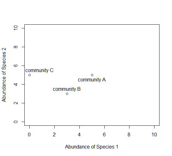
Now consider a third axis of abundance representing yet another species.
# install.packages("scatterplot3d")
library(scatterplot3d)
d=scatterplot3d(0:10,0:10,0:10,type="n",xlab="Abundance of Species 1",
  ylab="Abundance of Species 2",zlab="Abundance of Species 3"); d
d$points3d(5,5,0); text(d$xyz.convert(5,5,0.5),labels="community A")
d$points3d(3,3,3); text(d$xyz.convert(3,3,3.5),labels="community B")
d$points3d(0,5,5); text(d$xyz.convert(0,5,5.5),labels="community C")

Keep going, and imagine as many axes as there are species in these communities.

The goal of NMDS is to represent the original position of communities in multidimensional space as accurately as possible using a reduced number of dimensions that can be easily plotted and visualized (and to spare your thinker).
How does it work?
NMDS does not use the absolute abundances of species in communities, but rather their rank orders. The use of ranks omits some of the issues associated with using absolute distance (e.g., sensitivity to transformation), and as a result is much more flexible technique that accepts a variety of types of data. (It’s also where the “non-metric” part of the name comes from.)
The NMDS procedure is iterative and takes place over several steps:
- Define the original positions of communities in multidimensional space.
- Specify the number of reduced dimensions (typically 2).
- Construct an initial configuration of the samples in 2-dimensions.
- Regress distances in this initial configuration against the observed (measured) distances.
- Determine the stress, or the disagreement between 2-D configuration and predicted values from the regression. If the 2-D configuration perfectly preserves the original rank orders, then a plot of one against the other must be monotonically increasing. The extent to which the points on the 2-D configuration differ from this monotonically increasing line determines the degree of stress. This relationship is often visualized in what is called a Shepard plot.
- If stress is high, reposition the points in 2 dimensions in the direction of decreasing stress, and repeat until stress is below some threshold.**A good rule of thumb: stress < 0.05 provides an excellent representation in reduced dimensions, < 0.1 is great, < 0.2 is good/ok, and stress < 0.3 provides a poor representation.** To reiterate: high stress is bad, low stress is good!
Additional note: The final configuration may differ depending on the initial configuration (which is often random), and the number of iterations, so it is advisable to run the NMDS multiple times and compare the interpretation from the lowest stress solutions.
To begin, NMDS requires a distance matrix, or a matrix of dissimilarities. Raw Euclidean distances are not ideal for this purpose: they’re sensitive to total abundances, so may treat sites with a similar number of species as more similar, even though the identities of the species are different. They’re also sensitive to species absences, so may treat sites with the same number of absent species as more similar.
Consequently, ecologists use the Bray-Curtis dissimilarity calculation, which has a number of ideal properties:
- It is invariant to changes in units.
- It is unaffected by additions/removals of species that are not present in two communities,
- It is unaffected by the addition of a new community,
- It can recognize differences in total abundances when relative abundances are the same,
Let’s do it in R!
To run the NMDS, we will use the function metaMDS from the vegan package. The function requires only a community-by-species matrix (which we will create randomly).
You should see each iteration of the NMDS until a solution is reached (i.e., stress was minimized after some number of reconfigurations of the points in 2 dimensions). You can increase the number of default iterations using the argument trymax=. which may help alleviate issues of non-convergence. If high stress is your problem, increasing the number of dimensions to k=3 might also help.
example_NMDS=metaMDS(community_matrix,k=2,trymax=100)
You’ll see that metaMDS has automatically applied a square root transformation and calculated the Bray-Curtis distances for our community-by-site matrix.
Let’s examine a Shepard plot, which shows scatter around the regression between the interpoint distances in the final configuration (i.e., the distances between each pair of communities) against their original dissimilarities.
stressplot(example_NMDS)

Large scatter around the line suggests that original dissimilarities are not well preserved in the reduced number of dimensions. Looks pretty good in this case.
Now we can plot the NMDS. The plot shows us both the communities (“sites”, open circles) and species (red crosses), but we don’t know which circle corresponds to which site, and which species corresponds to which cross.
plot(example_NMDS)

We can use the function ordiplot and orditorp to add text to the plot in place of points to make some sense of this rather non-intuitive mess.
ordiplot(example_NMDS,type="n")
orditorp(example_NMDS,display="species",col="red",air=0.01)
orditorp(example_NMDS,display="sites",cex=1.25,air=0.01)

That’s it! There’s a few more tips and tricks I want to demonstrate.
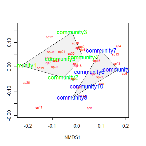
Let’s suppose that communities 1-5 had some treatment applied, and communities 6-10 a different treatment. We can draw convex hulls connecting the vertices of the points made by these communities on the plot. I find this an intuitive way to understand how communities and species cluster based on treatments.
treat=c(rep("Treatment1",5),rep("Treatment2",5))
ordiplot(example_NMDS,type="n")
ordihull(example_NMDS,groups=treat,draw="polygon",col="grey90",label=F)
orditorp(example_NMDS,display="species",col="red",air=0.01)
orditorp(example_NMDS,display="sites",col=c(rep("green",5),rep("blue",5)),
   air=0.01,cex=1.25)
One can also plot “spider graphs” using the function orderspider, ellipses using the function ordiellipse, or a minimum spanning tree (MST) using ordicluster which connects similar communities (useful to see if treatments are effective in controlling community structure).

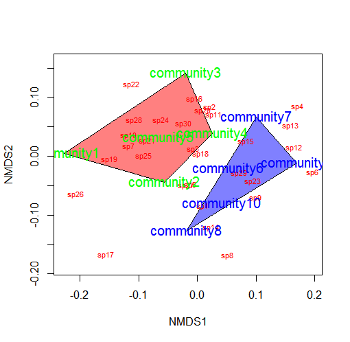
You could also color the convex hulls by treatment.
# First, create a vector of color values corresponding of the
# same length as the vector of treatment values
colors=c(rep("red",5),rep("blue",5))
ordiplot(example_NMDS,type="n")
#Plot convex hulls with colors baesd on treatment
for(i in unique(treat)) {
  ordihull(example_NMDS$point[grep(i,treat),],draw="polygon",
   groups=treat[treat==i],col=colors[grep(i,treat)],label=F) }
orditorp(example_NMDS,display="species",col="red",air=0.01)
orditorp(example_NMDS,display="sites",col=c(rep("green",5),
  rep("blue",5)),air=0.01,cex=1.25)
*You may wish to use a less garish color scheme than I
If the treatment is continuous, such as an environmental gradient, then it might be useful to plot contour lines rather than convex hulls. We can simply make up some, say, elevation data for our original community matrix and overlay them onto the NMDS plot using ordisurf:
Which produces the following plot:
 You could even do this for other continuous variables, such as temperature.
________________________
The full example code (annotated, with examples for the last several plots) is available below:
# Non-metric multidimensional scaling (NMDS) is one tool commonly used to
# examine community composition

# Let's lay some conceptual groundwork
# Consider a single axis of abundance representing a single species:
plot(0:10,0:10,type="n",axes=F,xlab="Abundance of Species 1",ylab="")
axis(1)
# We can plot each community on that axis depending on the abundance of
# species 1 within it
points(5,0); text(5.5,0.5,labels="community A")
points(3,0); text(3.2,0.5,labels="community B")
points(0,0); text(0.8,0.5,labels="community C")

# Now consider a second axis of abundance representing a different
# species
# Communities can be plotted along both axes depending on the abundance of
# species within it
plot(0:10,0:10,type="n",xlab="Abundance of Species 1",
     ylab="Abundance of Species 2")
points(5,5); text(5,4.5,labels="community A")
points(3,3); text(3,3.5,labels="community B")
points(0,5); text(0.8,5.5,labels="community C")

# Now consider a THIRD axis of abundance representing yet another species
# (For this we're going to need to load another package)
# install.packages("scatterplot3d")
library(scatterplot3d)
d=scatterplot3d(0:10,0:10,0:10,type="n",xlab="Abundance of Species 1",
                ylab="Abundance of Species 2",
                zlab="Abundance of Species 3"); d
d$points3d(5,5,0); text(d$xyz.convert(5,5,0.5),labels="community A")
d$points3d(3,3,3); text(d$xyz.convert(3,3,3.5),labels="community B")
d$points3d(0,5,5); text(d$xyz.convert(0,5,5.5),labels="community C")

# Now consider as many axes as there are species S (obviously we cannot
# visualize this beyond 3 dimensions)
# Hopefully your head didn't explode

# The goal of NMDS is to represent the original position of communities in
# multidimensional space as accurately as possible using a reduced number
# of dimensions that can be easily plotted and visualized

# NMDS does not use the absolute abundances of species in communities, but
# rather their RANK ORDER!
# The use of ranks omits some of the issues associated with using absolute
# distance (e.g., sensitivity to transformation), and as a result is much
# more flexible technique that accepts a variety of types of data
# (It is also where the "non-metric" part of the name comes from)

# The NMDS procedure is iterative and takes place over several steps:
# (1) Define the original positions of communities in multidimensional
# space
# (2) Specify the number m of reduced dimensions (typically 2)
# (3) Construct an initial configuration of the samples in 2-dimensions
# (4) Regress distances in this initial configuration against the observed
# (measured) distances
# (5) Determine the stress (disagreement between 2-D configuration and
# predicted values from regression)
# If the 2-D configuration perfectly preserves the original rank
# orders, then a plot ofone against the other must be monotonically
# increasing. The extent to which the points on the 2-D configuration
# differ from this monotonically increasing line determines the
# degree of stress (see Shepard plot)
# (6) If stress is high, reposition the points in m dimensions in the
#direction of decreasing stress, and repeat until stress is below
#some threshold

# Generally, stress < 0.05 provides an excellent represention in reduced
# dimensions, < 0.1 is great, < 0.2 is good, and stress > 0.3 provides a
# poor representation

# NOTE: The final configuration may differ depending on the initial
# configuration (which is often random) and the number of iterations, so
# it is advisable to run the NMDS multiple times and compare the
# interpretation from the lowest stress solutions

# To begin, NMDS requires a distance matrix, or a matrix of
# dissimilarities
# Raw Euclidean distances are not ideal for this purpose: they are
# sensitive to totalabundances, so may treat sites with a similar number
# of species as more similar, even though the identities of the species
# are different
# They are also sensitive to species absences, so may treat sites with
# the same number of absent species as more similar

# Consequently, ecologists use the Bray-Curtis dissimilarity calculation,
# which has many ideal properties:
# It is invariant to changes in units
# It is unaffected by additions/removals of species that are not
# present in two communities
# It is unaffected by the addition of a new community
# It can recognize differences in total abudnances when relative
# abundances are the same

# To run the NMDS, we will use the function `metaMDS` from the vegan
# package
#install.packages("vegan")
library(vegan)
# `metaMDS` requires a community-by-species matrix
# Let's create that matrix with some randomly sampled data
set.seed(2)
community_matrix=matrix(sample(1:100,300,replace=T),nrow=10,
                        dimnames=list(paste("community",1:10,sep=""),
                                      paste("sp",1:30,sep="")))

# The function `metaMDS` will take care of most of the distance
# calculations, iterative fitting, etc. We need simply to supply:
example_NMDS=metaMDS(community_matrix, # Our community-by-species matrix
                     k=2) # The number of reduced dimensions
# You should see each iteration of the NMDS until a solution is reached
# (i.e., stress was minimized after some number of reconfigurations of
# the points in 2 dimensions). You can increase the number of default
# iterations using the argument "trymax=##"
example_NMDS=metaMDS(community_matrix,k=2,trymax=100)

# And we can look at the NMDS object
example_NMDS # metaMDS has automatically applied a square root
# transformation and calculated the Bray-Curtis distances for our
# community-by-site matrix
# Let's examine a Shepard plot, which shows scatter around the regression
# between the interpoint distances in the final configuration (distances
# between each pair of communities) against their original dissimilarities
stressplot(example_NMDS)
# Large scatter around the line suggests that original dissimilarities are
# not well preserved in the reduced number of dimensions

#Now we can plot the NMDS
plot(example_NMDS)
# It shows us both the communities ("sites", open circles) and species
# (red crosses), but we  don't know which are which!

# We can use the functions `ordiplot` and `orditorp` to add text to the
# plot in place of points
ordiplot(example_NMDS,type="n")
orditorp(example_NMDS,display="species",col="red",air=0.01)
orditorp(example_NMDS,display="sites",cex=1.25,air=0.01)

# There are some additional functions that might of interest
# Let's suppose that communities 1-5 had some treatment applied, and
# communities 6-10 a different treatment
# We can draw convex hulls connecting the vertices of the points made by
# these communities on the plot
# First, let's create a vector of treatment values:
treat=c(rep("Treatment1",5),rep("Treatment2",5))
ordiplot(example_NMDS,type="n")
ordihull(example_NMDS,groups=treat,draw="polygon",col="grey90",
         label=FALSE)
orditorp(example_NMDS,display="species",col="red",air=0.01)
orditorp(example_NMDS,display="sites",col=c(rep("green",5),rep("blue",5)),
         air=0.01,cex=1.25)
# I find this an intuitive way to understand how communities and species
# cluster based on treatments
# One can also plot ellipses and "spider graphs" using the functions
# `ordiellipse` and `orderspider` which emphasize the centroid of the
# communities in each treatment

# Another alternative is to plot a minimum spanning tree (from the
# function `hclust`), which clusters communities based on their original
# dissimilarities and projects the dendrogram onto the 2-D plot
ordiplot(example_NMDS,type="n")
orditorp(example_NMDS,display="species",col="red",air=0.01)
orditorp(example_NMDS,display="sites",col=c(rep("green",5),rep("blue",5)),
         air=0.01,cex=1.25)
ordicluster(example_NMDS,hclust(vegdist(community_matrix,"bray")))
# Note that clustering is based on Bray-Curtis distances
# This is one method suggested to check the 2-D plot for accuracy

# You could also plot the convex hulls, ellipses, spider plots, etc. colored based on the treatments
# First, create a vector of color values corresponding of the same length as the vector of treatment values
colors=c(rep("red",5),rep("blue",5))
ordiplot(example_NMDS,type="n")
#Plot convex hulls with colors baesd on treatment
for(i in unique(treat)) {
  ordihull(example_NMDS$point[grep(i,treat),],draw="polygon",groups=treat[treat==i],col=colors[grep(i,treat)],label=F) }
orditorp(example_NMDS,display="species",col="red",air=0.01)
orditorp(example_NMDS,display="sites",col=c(rep("green",5),rep("blue",5)),
         air=0.01,cex=1.25)

# If the treatment is a continuous variable, consider mapping contour
# lines onto the plot
# For this example, consider the treatments were applied along an
# elevational gradient
# We can define random elevations for previous example
elevation=runif(10,0.5,1.5)
# And use the function ordisurf to plot contour lines
ordisurf(example_NMDS,elevation,main="",col="forestgreen")
# Finally, we want to display species on plot
orditorp(example_NMDS,display="species",col="grey30",air=0.1,cex=1)

Thank you so much, this has been invaluable!